Chapter 8 — Diagonalization
Linear Algebra and its Applications · IISc 2024 · typeset reproduction
For this chapter, \( \F = \C \). \( P_{\F} \) denotes the space of polynomials with complex coefficients.
Diagonalizable Operators
Definition 39 — Diagonalizable
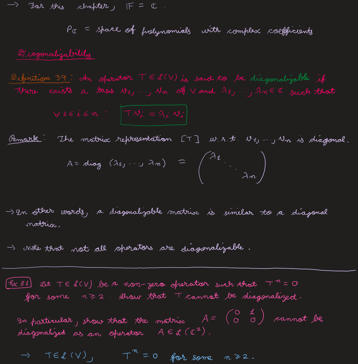
An operator \( T \in \Lin(V) \) is diagonalizable if there is a basis \( v_1, \dots, v_n \) of \(V\) and scalars \( \lambda_1, \dots, \lambda_n \in \F \) such that \( T v_i = \lambda_i v_i \) for all \(i\). The matrix representation w.r.t. \( v_1, \dots, v_n \) is then diagonal, \( A = \diag(\lambda_1, \dots, \lambda_n) \). In other words, a diagonalizable matrix is similar to a diagonal matrix. Not all operators are diagonalizable.
Ex 81
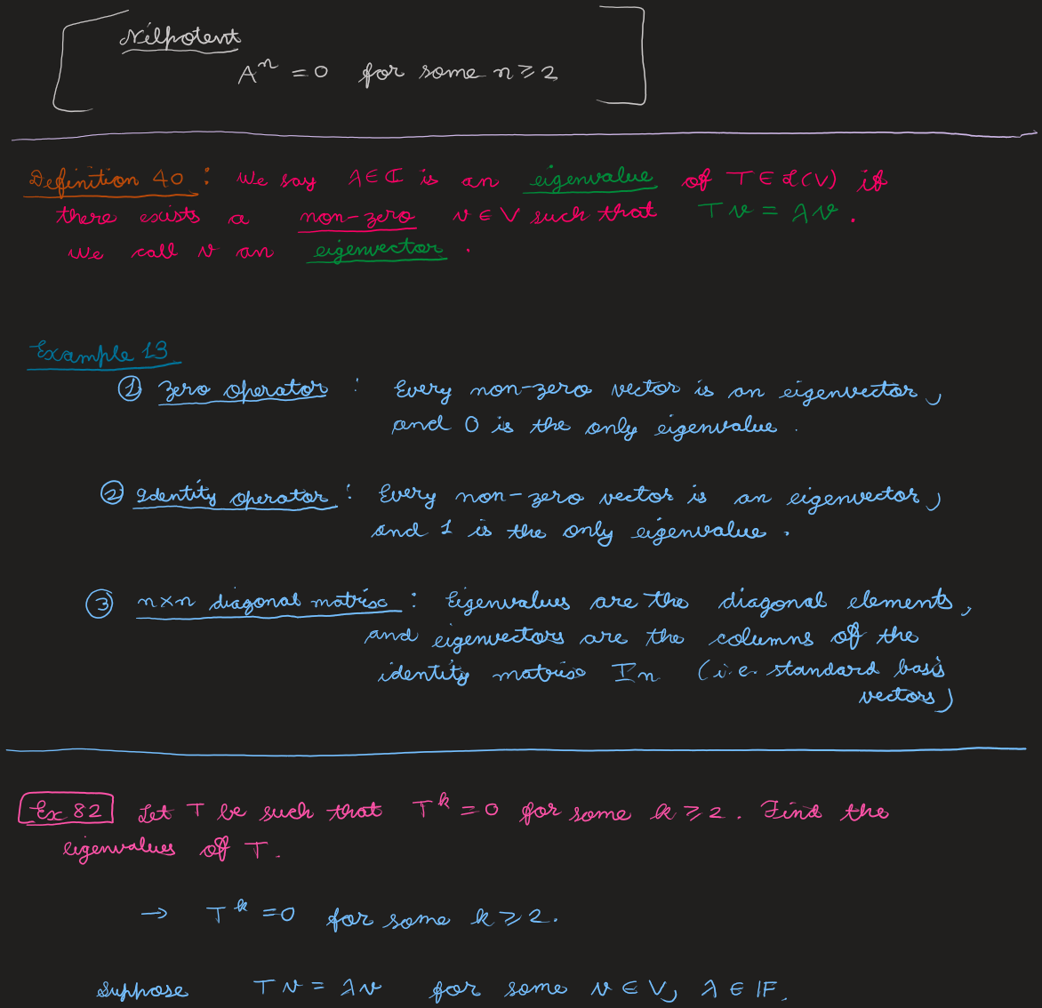
Let \( T \in \Lin(V) \) be a non-zero operator with \( T^n = 0 \) for some \( n \ge 2 \) (nilpotent). Show that \(T\) cannot be diagonalized. In particular, the matrix \( A = \begin{bmatrix} 0 & 1 \\ 0 & 0 \end{bmatrix} \) cannot be diagonalized as an operator \( A \in \Lin(\C^2) \).
Solution
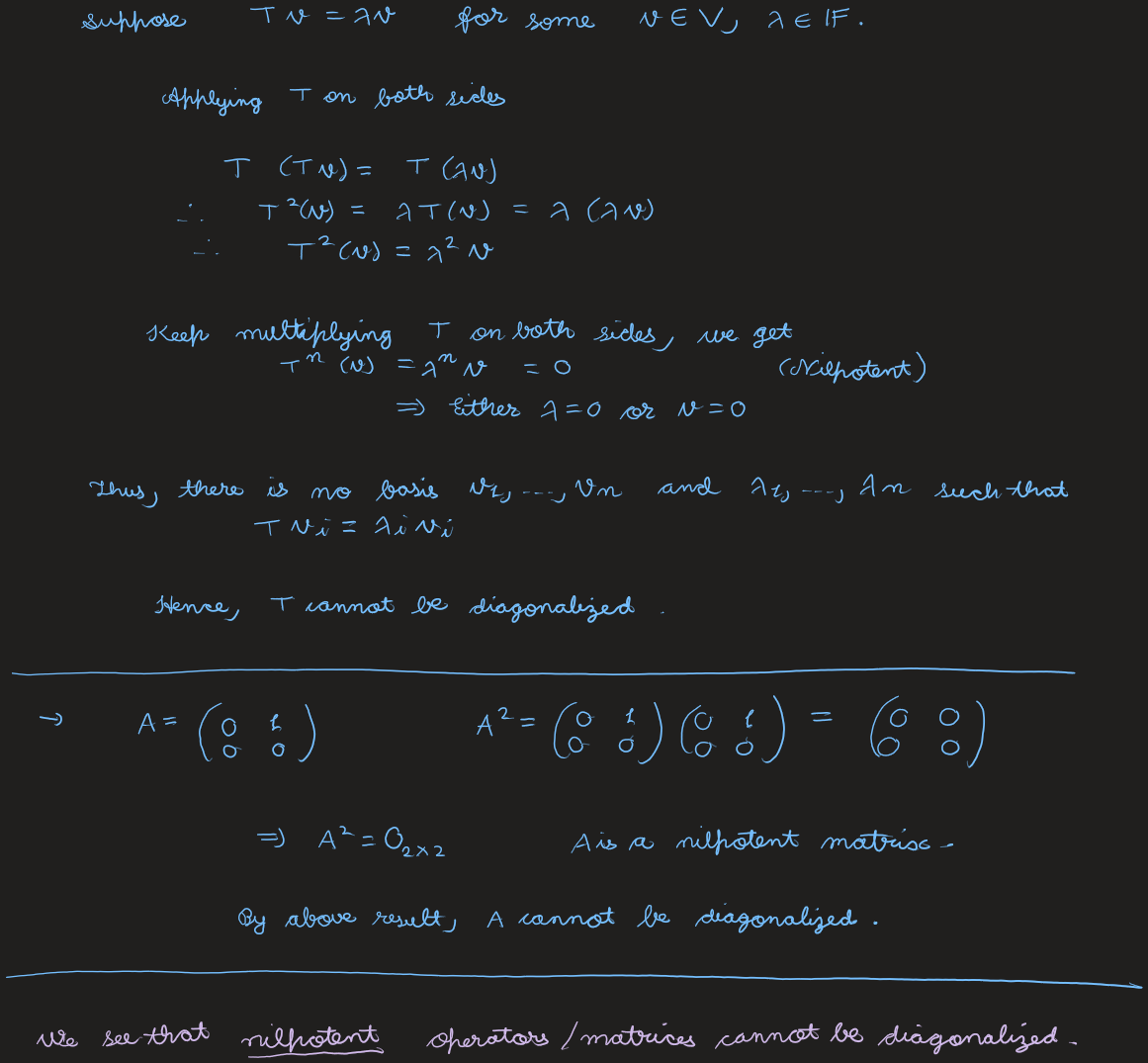
Suppose \( Tv = \lambda v \) for some \( v \in V \), \( \lambda \in \F \). Applying \(T\) repeatedly, \( T^2 v = \lambda T(v) = \lambda^2 v \), and \( T^n(v) = \lambda^n v = 0 \) (nilpotent), so either \( \lambda = 0 \) or \( v = 0 \) — every eigenvalue of \(T\) is \(0\). A diagonalizable \(T\) would then be similar to \( \diag(0,\dots,0) = O \), forcing \( T = 0 \) and contradicting \( T \neq 0 \). So \(T\) cannot be diagonalized.
For \( A = \begin{bmatrix} 0 & 1 \\ 0 & 0 \end{bmatrix} \), \( A^2 = \begin{bmatrix} 0 & 1 \\ 0 & 0 \end{bmatrix}\begin{bmatrix} 0 & 1 \\ 0 & 0 \end{bmatrix} = \begin{bmatrix} 0 & 0 \\ 0 & 0 \end{bmatrix} = O_{2\times 2} \), so \(A\) is nilpotent and, by the above, cannot be diagonalized. (Nilpotent operators/matrices cannot be diagonalized.)
Eigenvalues & Eigenvectors
Definition 40 — Eigenvalue / eigenvector
\( \lambda \in \F \) is an eigenvalue of \( T \in \Lin(V) \) if there is a non-zero \( v \in V \) with \( Tv = \lambda v \); such a \(v\) is an eigenvector.
Example 13
- Zero operator: every non-zero vector is an eigenvector, and \(0\) is the only eigenvalue.
- Identity operator: every non-zero vector is an eigenvector, and \(1\) is the only eigenvalue.
- \( n\times n \) diagonal matrix: the eigenvalues are the diagonal elements, and the eigenvectors are the columns of \( I_n \) (the standard basis vectors).
Ex 82
Let \(T\) satisfy \( T^k = 0 \) for some \( k \ge 2 \). Find the eigenvalues of \(T\).
Solution
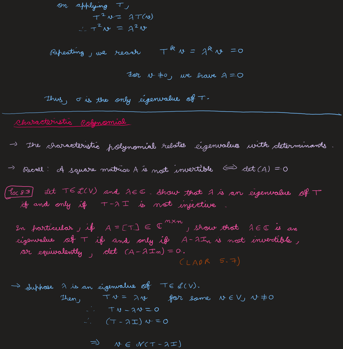
Suppose \( Tv = \lambda v \), \( v \neq 0 \). Applying \(T\), \( T^2 v = \lambda^2 v \), and repeating, \( T^k v = \lambda^k v = 0 \). For \( v \neq 0 \), \( \lambda = 0 \). Thus \(0\) is the only eigenvalue of \(T\).
Characteristic Polynomial
The characteristic polynomial relates eigenvalues with determinants. Recall: a square matrix \(A\) is not invertible \( \iff \det(A) = 0 \).
Ex 83
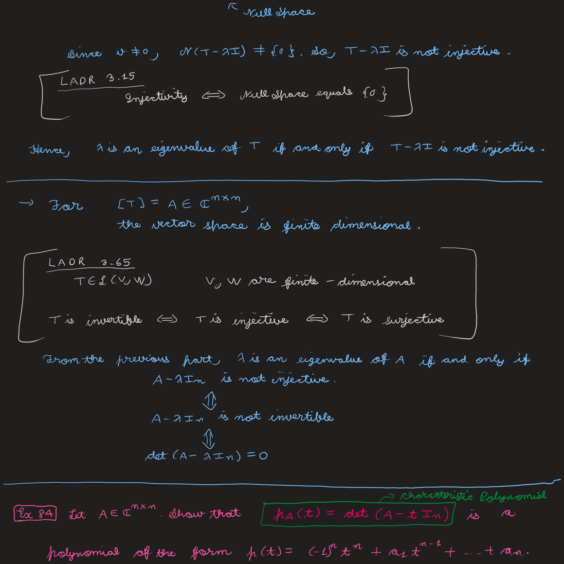
Let \( T \in \Lin(V) \) and \( \lambda \in \C \). Show that \( \lambda \) is an eigenvalue of \(T\) iff \( T - \lambda I \) is not injective. In particular, if \( A = [T] \in \C^{n\times n} \), \( \lambda \in \C \) is an eigenvalue iff \( A - \lambda I \) is not invertible, equivalently \( \det(A - \lambda I_n) = 0 \). (LADR 5.7)
Solution
If \( \lambda \) is an eigenvalue, \( Tv = \lambda v \) for some \( v \neq 0 \), so \( (T - \lambda I)v = 0 \), i.e. \( v \in \Null(T - \lambda I) \). Since \( v \neq 0 \), \( \Null(T - \lambda I) \neq \{0\} \), so \( T - \lambda I \) is not injective (LADR 3.16: injectivity \( \iff \) null space \( = \{0\} \)). Conversely the same chain runs backwards. For \( [T] = A \in \C^{n\times n} \) (finite-dimensional), \( T - \lambda I \) is invertible \( \iff \) injective \( \iff \) surjective (LADR 3.65), so \( \lambda \) is an eigenvalue \( \iff A - \lambda I \) is not invertible \( \iff \det(A - \lambda I) = 0 \).
Ex 84
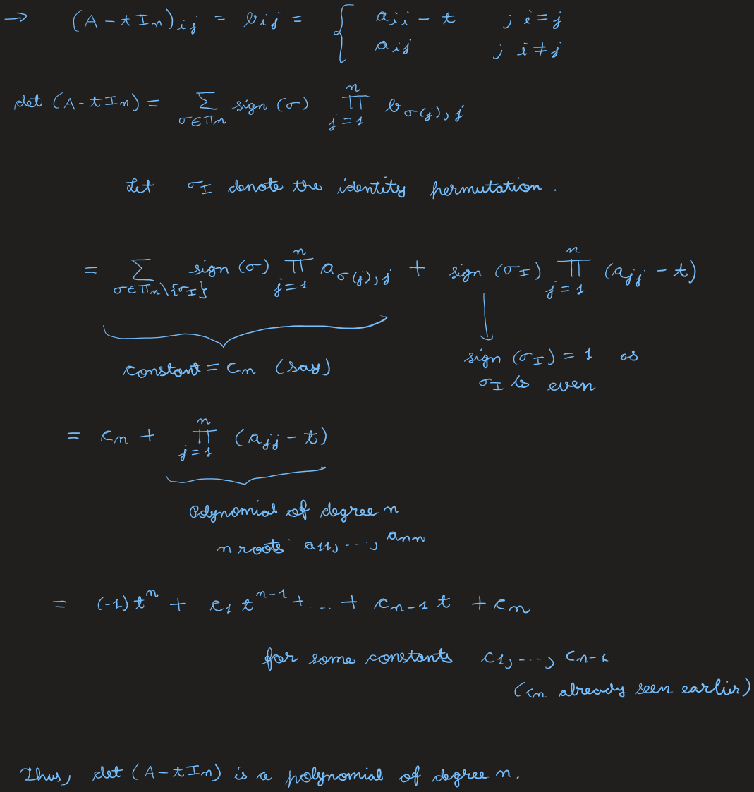
Let \( A \in \C^{n\times n} \). Show that \( p(\lambda) = \det(A - \lambda I) \) is a polynomial of the form \( p(\lambda) = (-1)^n\lambda^n + a_{n-1}\lambda^{n-1} + \dots + a_1\lambda + a_0 \).
Solution
With \( (A - tI_n)_{ij} = b_{ij} = \begin{cases} a_{ii} - t & i = j \\ a_{ij} & i \neq j \end{cases} \), the Leibniz formula gives \( \det(A - tI_n) = \sum_{\sigma\in\Pi_n}\sign(\sigma)\prod_{j=1}^{n}b_{\sigma(j),j} \). Splitting off the identity permutation \( \sigma_I \) (with \( \sign(\sigma_I) = 1 \)), \[ \det(A - tI_n) = \underbrace{\sum_{\sigma\in\Pi_n\setminus\{\sigma_I\}}\sign(\sigma)\prod_{j=1}^{n}a_{\sigma(j),j}}_{\text{lower-degree terms}} + \prod_{j=1}^{n}(a_{jj} - t), \] where \( \prod_{j=1}^{n}(a_{jj} - t) \) is a degree-\(n\) polynomial (roots \( a_{11}, \dots, a_{nn} \)). Collecting terms, \[ \det(A - tI_n) = (-1)^n t^n + c_1 t^{n-1} + \dots + c_{n-1}t + c_n \] for some constants. Thus \( \det(A - tI_n) \) is a polynomial of degree \(n\).
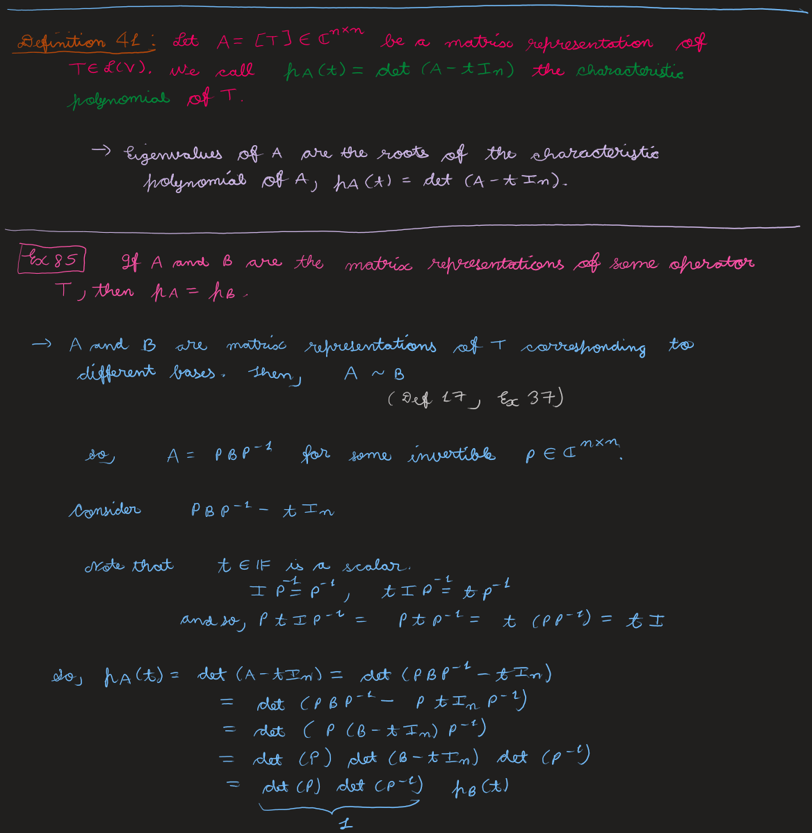
Definition 41 — Characteristic polynomial
The eigenvalues of \(A\) are the roots of the characteristic polynomial \( f_A(\lambda) = \det(A - \lambda I_n) \).
Ex 85
If \(A\) and \(B\) are the matrix representations of the same operator \(T\), then \( f_A = f_B \) (the eigenvalues do not depend on the choice of basis).
Solution
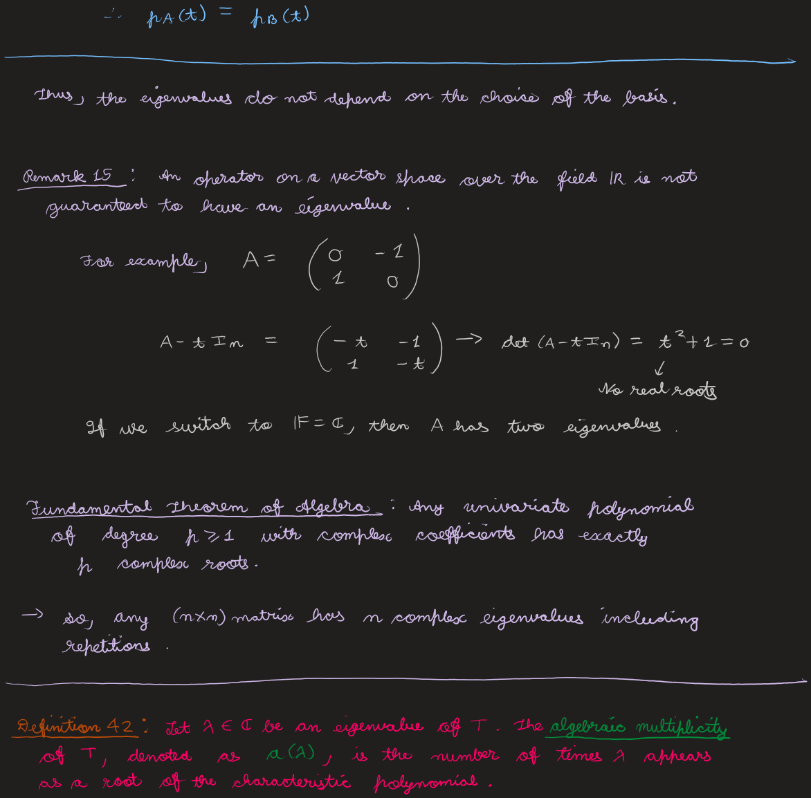
\(A\) and \(B\) represent \(T\) in different bases, so \( A \sim B \) (Ex 37), i.e. \( A = PBP^{-1} \) for some invertible \(P\). Since \( P(tI)P^{-1} = tI \), \[\begin{aligned} f_A(\lambda) &= \det(A - \lambda I) = \det(PBP^{-1} - \lambda PIP^{-1}) \\ &= \det\!\big(P(B - \lambda I)P^{-1}\big) \\ &= \det(P)\det(B - \lambda I)\det(P^{-1}) \\ &= \det(B - \lambda I) = f_B(\lambda). \end{aligned}\]
Remark
An operator over \( \R \) need not have an eigenvalue. E.g. \( A = \begin{bmatrix} 0 & -1 \\ 1 & 0 \end{bmatrix} \) gives \( \det(A - tI) = t^2 + 1 = 0 \), which has no real roots; over \( \C \) it has two eigenvalues. By the Fundamental Theorem of Algebra, any univariate polynomial of degree \( p \ge 1 \) with complex coefficients has exactly \(p\) complex roots, so any \( n\times n \) matrix has \(n\) complex eigenvalues (including repetitions).
Definition 42 — Algebraic multiplicity
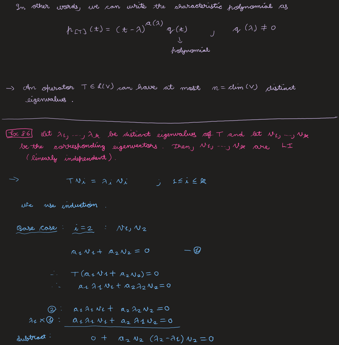
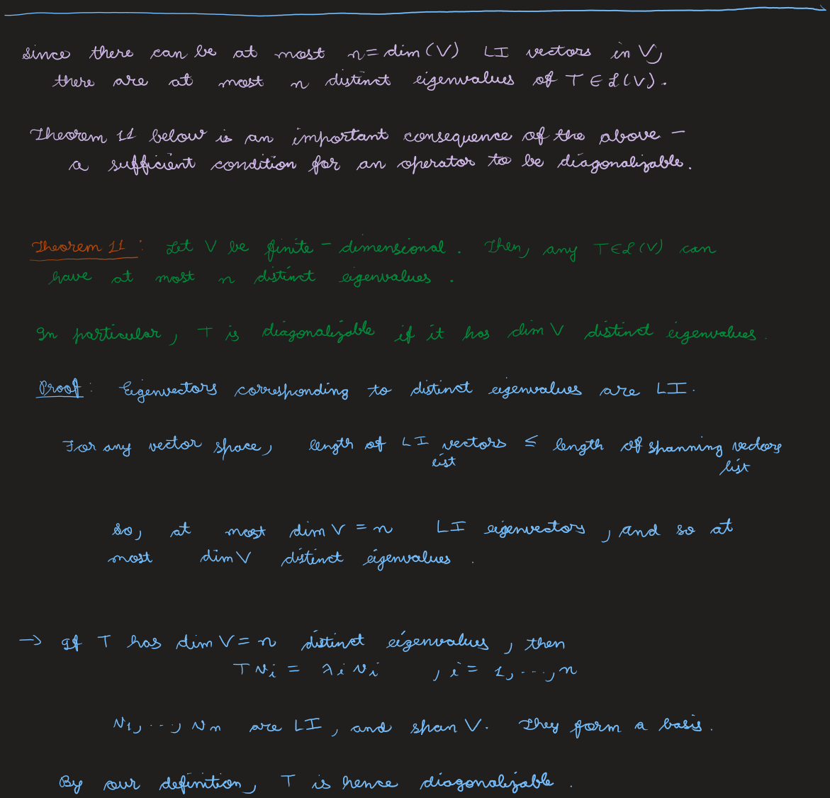
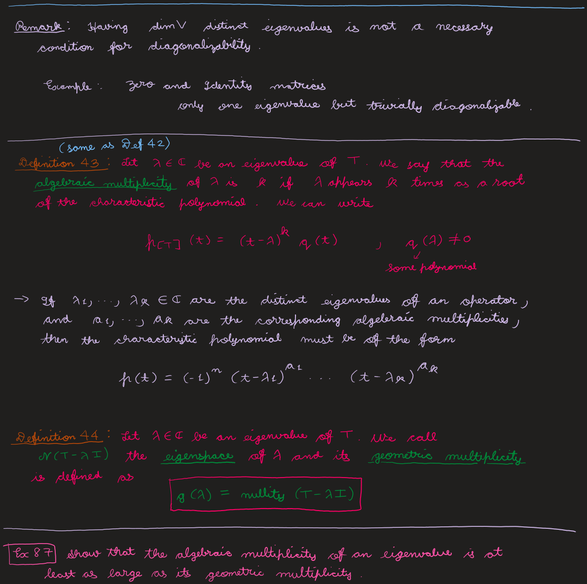
Let \( \lambda \in \C \) be an eigenvalue of \(T\). The algebraic multiplicity \( a(\lambda) \) is the number of times \( \lambda \) appears as a root of the characteristic polynomial: \( f_{[T]}(t) = (t - \lambda)^{a(\lambda)}q(t) \), \( q(\lambda) \neq 0 \). If \( \lambda_1, \dots, \lambda_k \) are the distinct eigenvalues with multiplicities \( a_1, \dots, a_k \), then \( p(\lambda) = (-1)^n(\lambda - \lambda_1)^{a_1}\cdots(\lambda - \lambda_k)^{a_k} \). An operator has at most \( n = \dim V \) distinct eigenvalues.
Ex 86
Let \( \lambda_1, \dots, \lambda_k \) be distinct eigenvalues of \(T\) with corresponding eigenvectors \( v_1, \dots, v_k \). Then \( v_1, \dots, v_k \) are linearly independent.
Solution
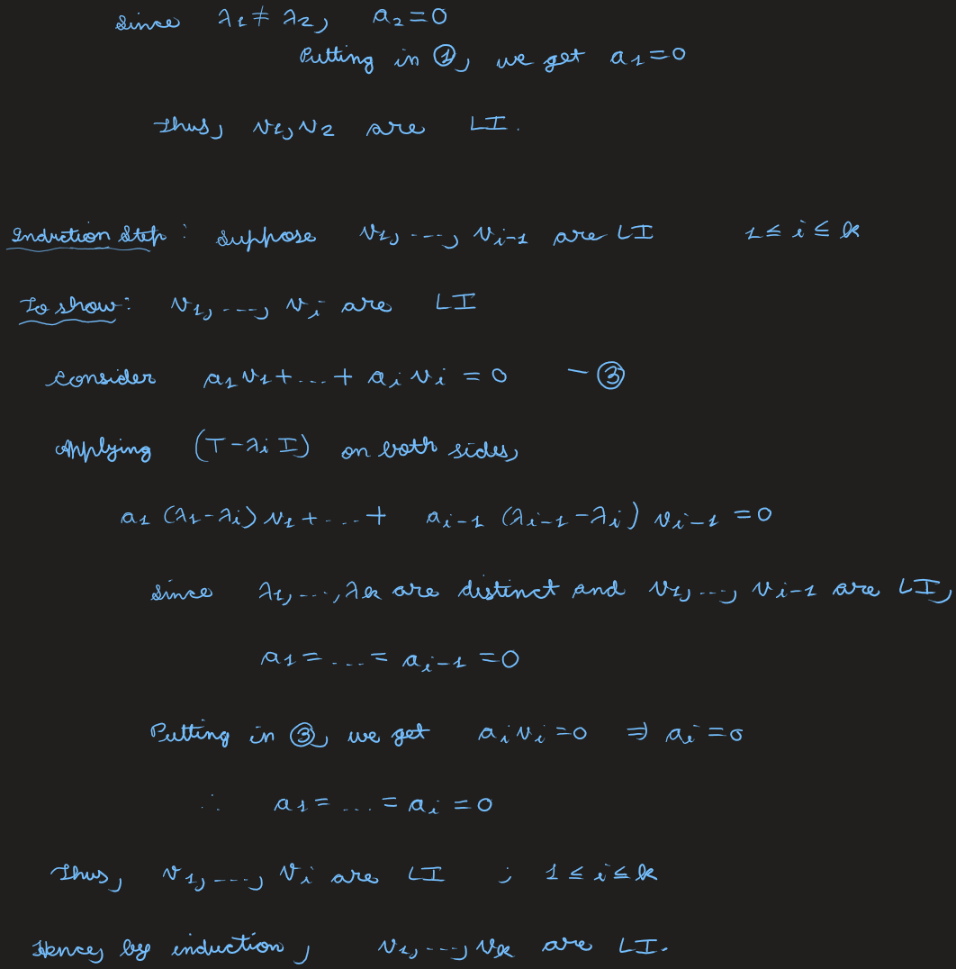
By induction. Base case \( i = 2 \): from \( a_1 v_1 + a_2 v_2 = 0 \) (①), apply \(T\): \( a_1\lambda_1 v_1 + a_2\lambda_2 v_2 = 0 \) (②). Compute \( \lambda_1\cdot① - ② \): \( a_2 v_2(\lambda_2 - \lambda_1) = 0 \); since \( \lambda_1 \neq \lambda_2 \), \( a_2 = 0 \), and then \( a_1 = 0 \). So \( v_1, v_2 \) are LI.
Inductive step. Assume \( v_1, \dots, v_{i-1} \) are LI. From \( a_1 v_1 + \dots + a_i v_i = 0 \) (③), apply \( (T - \lambda_i I) \): \[ a_1(\lambda_1 - \lambda_i)v_1 + \dots + a_{i-1}(\lambda_{i-1} - \lambda_i)v_{i-1} = 0. \] Since the \( \lambda_j \) are distinct and \( v_1, \dots, v_{i-1} \) are LI, \( a_1 = \dots = a_{i-1} = 0 \); putting back in ③, \( a_i v_i = 0 \Rightarrow a_i = 0 \). So \( v_1, \dots, v_i \) are LI, and by induction \( v_1, \dots, v_k \) are LI.
Theorem 11
If \(V\) is finite-dimensional, any \( T \in \Lin(V) \) with \( n = \dim(V) \) distinct eigenvalues is diagonalizable.
Proof
Eigenvectors corresponding to distinct eigenvalues are LI (Ex 86). With \(n\) distinct eigenvalues we get \(n\) LI eigenvectors, which form a basis of \(V\); hence \(T\) is diagonalizable. (This is a corollary of Theorem 12 below.)
Definition 43 — Geometric multiplicity
Let \( \lambda \in \C \) be an eigenvalue of \(T\). The geometric multiplicity is \( g(\lambda) = \nullity(T - \lambda I) = \dim\Null(A - \lambda I) \).
Correction — definition numbering
The instructor's notes define algebraic multiplicity twice (Def 42 and a near-identical Def 43); these notes keep it once (Def 42), so geometric multiplicity is Def 43 here (it is Def 44 in the instructor's PDF), and the matrix polynomial below is Def 44 here (left unnumbered by the instructor). The global count is unaffected — Chapter 9 still begins at Def 45.
Ex 87
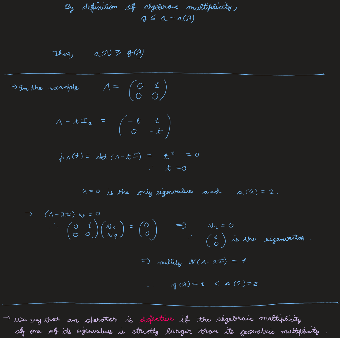
Show that the algebraic multiplicity of an eigenvalue is at least its geometric multiplicity, \( a(\lambda) \ge g(\lambda) \). Moreover, using \( A = \begin{bmatrix} 0 & 1 \\ 0 & 0 \end{bmatrix} \), show the algebraic multiplicity can be strictly larger than the geometric.
Solution
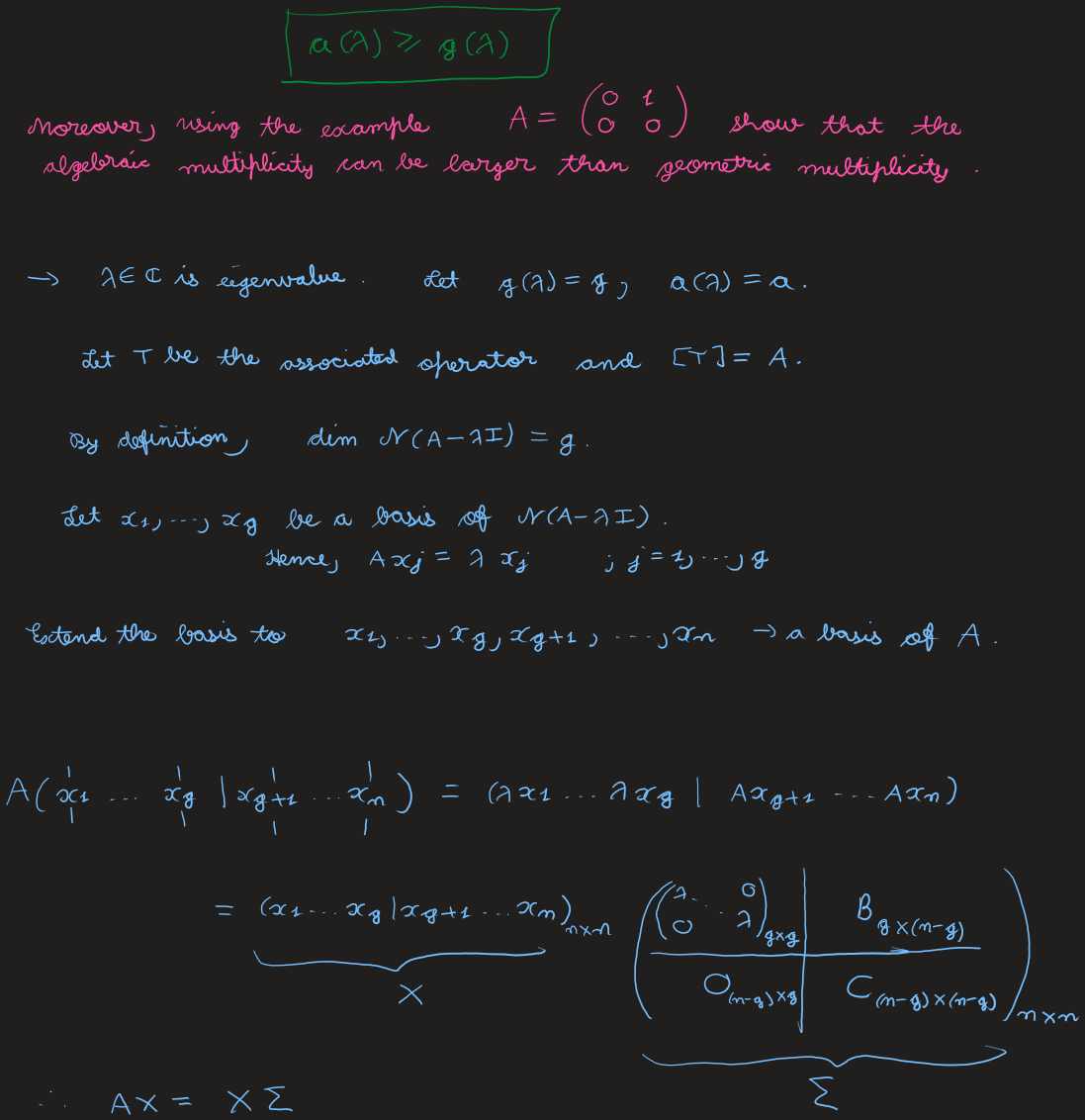
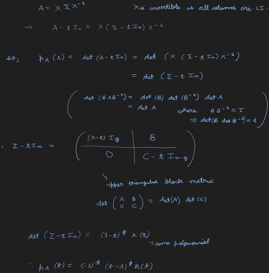
Let \( g = g(\lambda) \), \( a = a(\lambda) \), \( [T] = A \), \( \dim\Null(A - \lambda I) = g \). Let \( x_1, \dots, x_g \) be a basis of \( \Null(A - \lambda I) \) (so \( Ax_j = \lambda x_j \)), and extend to a basis \( x_1, \dots, x_g, x_{g+1}, \dots, x_n \) of \( \C^n \). Then \[ A\,[\,x_1 \cdots x_g \mid x_{g+1} \cdots x_n\,] = [\,x_1 \cdots x_n\,]\underbrace{\begin{bmatrix} \lambda I_g & B \\ O & C \end{bmatrix}}_{\Sigma}, \qquad AX = X\Sigma, \] so \( A = X\Sigma X^{-1} \) (\(X\) invertible as its columns are LI). Then \[\begin{aligned} f_A(t) &= \det(A - tI_n) = \det\!\big(X(\Sigma - tI_n)X^{-1}\big) \\ &= \det(\Sigma - tI_n) \\ &= \det\begin{bmatrix} (\lambda - t)I_g & B \\ O & C - tI_{n-g} \end{bmatrix} = (\lambda - t)^g\,h(t), \end{aligned}\] using \( \det\begin{bmatrix} A & B \\ O & C \end{bmatrix} = \det(A)\det(C) \). So \( f_A(t) = (-1)^g(t - \lambda)^g h(t) \), and by the definition of algebraic multiplicity \( g \le a \), i.e. \( a(\lambda) \ge g(\lambda) \).
For \( A = \begin{bmatrix} 0 & 1 \\ 0 & 0 \end{bmatrix} \): \( f_A(t) = t^2 = 0 \), so \( \lambda = 0 \) with \( a(\lambda) = 2 \). From \( (A - \lambda I)v = 0 \), \( v_2 = 0 \), so \( \begin{bmatrix} 1 \\ 0 \end{bmatrix} \) is the only eigenvector direction, \( \nullity(A - \lambda I) = 1 \), giving \( g(\lambda) = 1 < a(\lambda) = 2 \). An operator is defective if some eigenvalue has algebraic multiplicity strictly larger than its geometric multiplicity.
View original handwritten scans — Diagonalizability, eigenvalues & characteristic polynomial (pages 1–15)
Complete Characterization of Diagonalizability
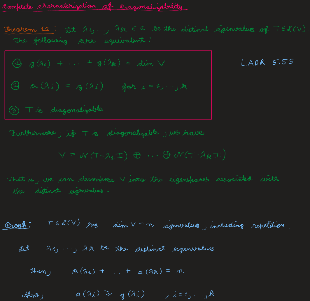
Theorem 12 — LADR 5.55
Let \( \lambda_1, \dots, \lambda_k \in \C \) be the distinct eigenvalues of \( T \in \Lin(V) \). The following are equivalent:
- \( g(\lambda_1) + \dots + g(\lambda_k) = \dim V \).
- \( a(\lambda_i) = g(\lambda_i) \) for \( i = 1, \dots, k \).
- \(T\) is diagonalizable.
Furthermore, if \(T\) is diagonalizable, \( V = \Null(T - \lambda_1 I) \oplus \dots \oplus \Null(T - \lambda_k I) \) — \(V\) decomposes into the eigenspaces of the distinct eigenvalues.
Proof
\(T\) has \( \dim V = n \) eigenvalues (with repetition); let \( \lambda_1, \dots, \lambda_k \) be distinct, so \( a(\lambda_1) + \dots + a(\lambda_k) = n \) and \( a(\lambda_i) \ge g(\lambda_i) \).
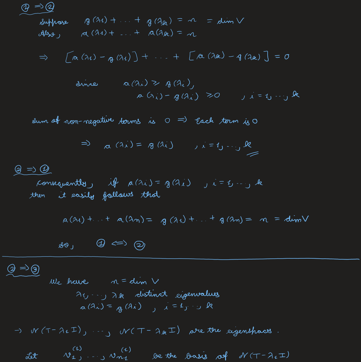
(1) \( \Rightarrow \) (2). If \( g(\lambda_1) + \dots + g(\lambda_k) = n \), then \( \sum_i[a(\lambda_i) - g(\lambda_i)] = 0 \) with each term \( \ge 0 \), so each \( a(\lambda_i) = g(\lambda_i) \). (2) \( \Rightarrow \) (1) follows since \( \sum a(\lambda_i) = \sum g(\lambda_i) = n \).
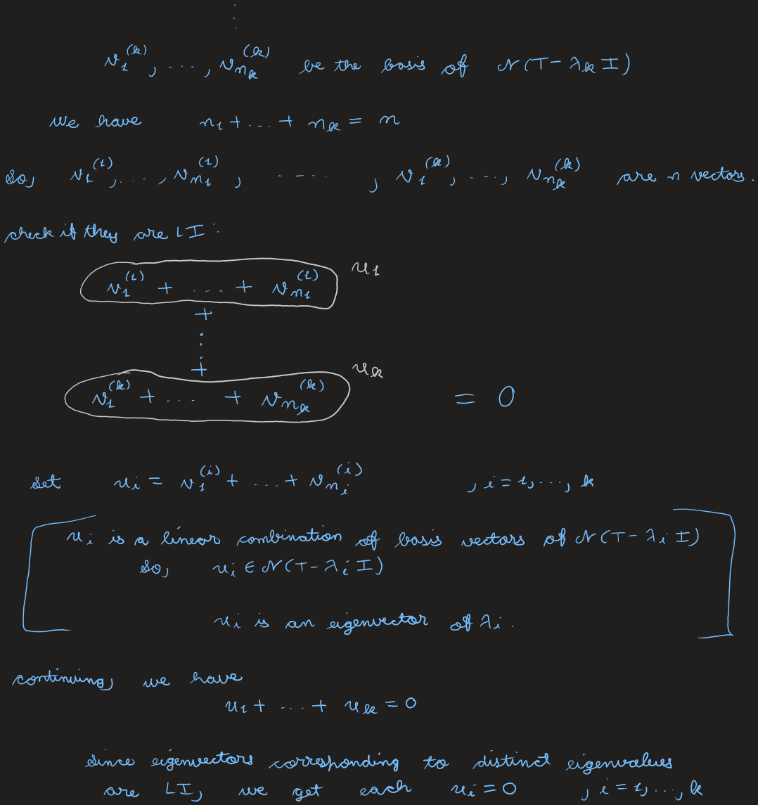
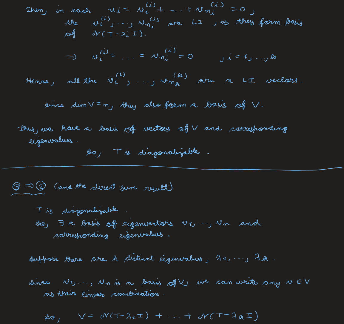
(2) \( \Rightarrow \) (3). Take bases \( v_1^{(i)}, \dots, v_{n_i}^{(i)} \) of each eigenspace \( \Null(T - \lambda_i I) \), with \( n_1 + \dots + n_k = n \). To check the \(n\) vectors are LI, set \( u_i = v_1^{(i)} + \dots + v_{n_i}^{(i)} \in \Null(T - \lambda_i I) \) (an eigenvector for \( \lambda_i \)). From \( u_1 + \dots + u_k = 0 \) and LI of eigenvectors for distinct eigenvalues, each \( u_i = 0 \); then within each eigenspace the \( v_j^{(i)} \) are LI, so all coefficients vanish. Hence the \(n\) vectors are LI, forming a basis of eigenvectors, so \(T\) is diagonalizable.
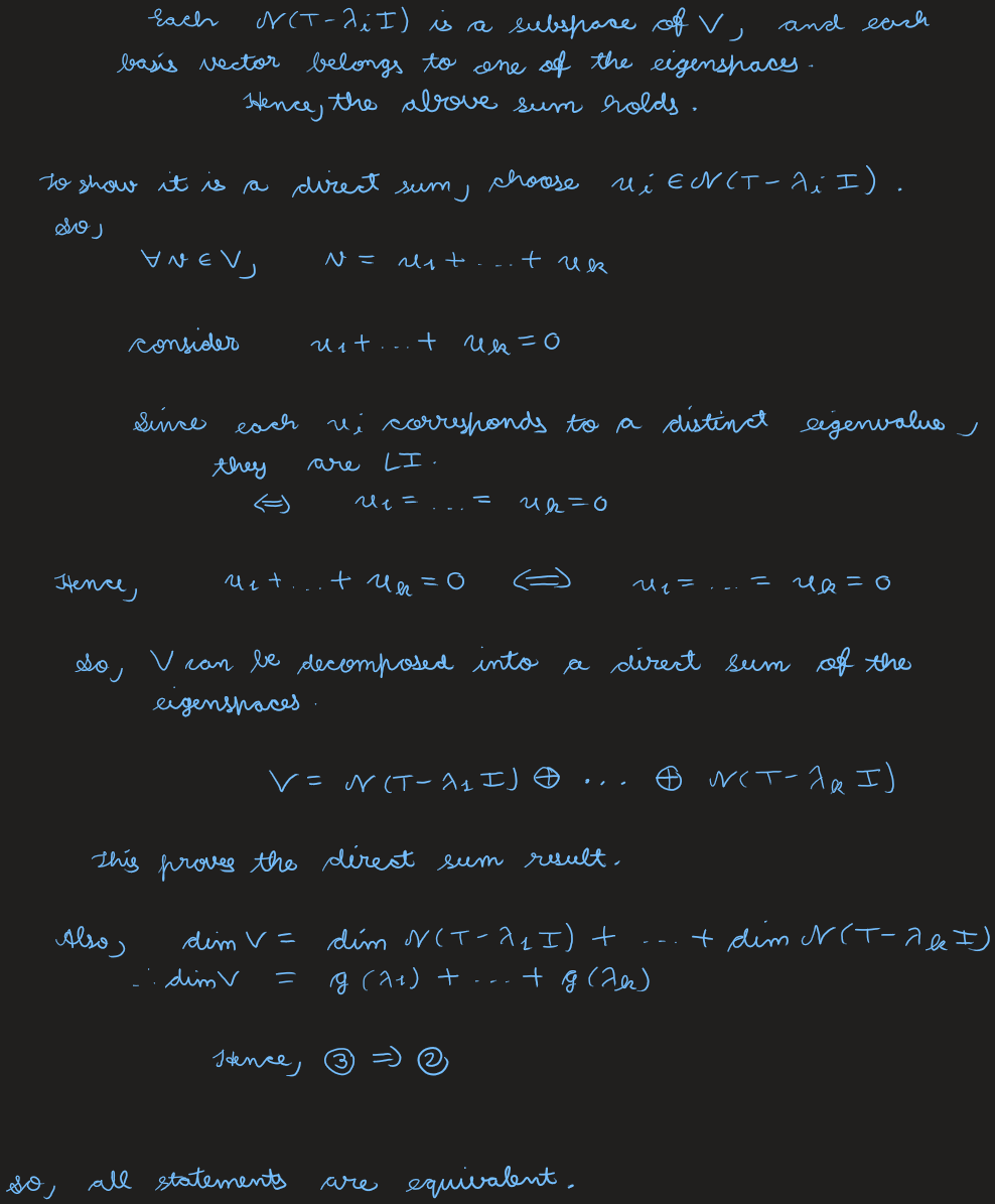
(3) \( \Rightarrow \) (2) (with the direct sum). If \(T\) is diagonalizable there is a basis of eigenvectors, so \( V = \Null(T - \lambda_1 I) + \dots + \Null(T - \lambda_k I) \). To see the sum is direct, take \( u_i \in \Null(T - \lambda_i I) \); \( u_1 + \dots + u_k = 0 \iff u_1 = \dots = u_k = 0 \) (LI of distinct-eigenvalue eigenvectors), so \( V = \bigoplus_i \Null(T - \lambda_i I) \) and \( \dim V = \sum_i g(\lambda_i) \). Hence all three are equivalent.
Ex 88
Let \( \lambda_1, \dots, \lambda_k \) be the distinct eigenvalues of \(T\) and \( u_i \in \Null(T - \lambda_i I) \). Prove \( u_1 + \dots + u_k = 0 \iff u_1 = \dots = u_k = 0 \).
Solution
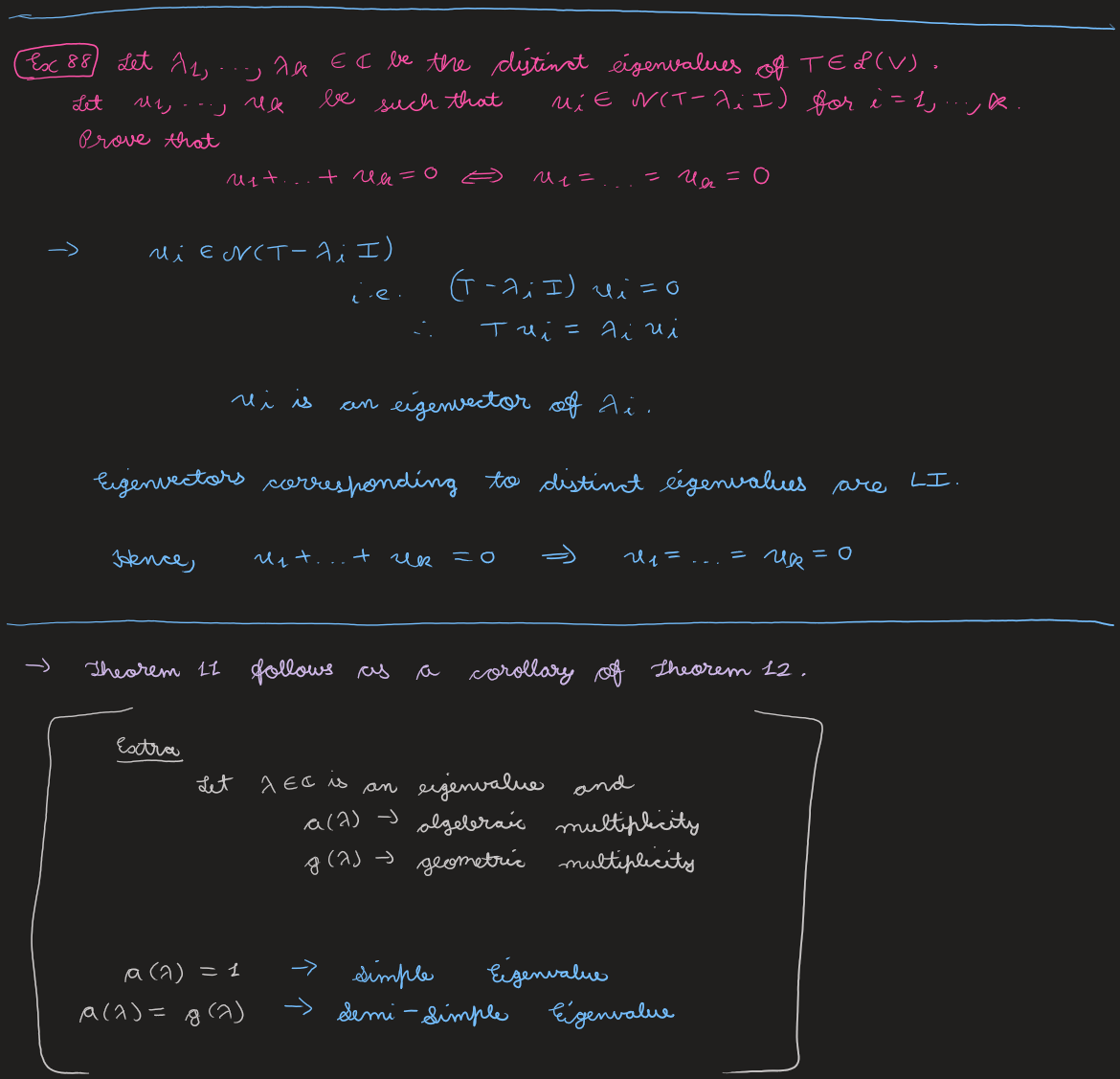
\( u_i \in \Null(T - \lambda_i I) \) means \( (T - \lambda_i I)u_i = 0 \), i.e. \( Tu_i = \lambda_i u_i \), so each non-zero \( u_i \) is an eigenvector for \( \lambda_i \). Eigenvectors for distinct eigenvalues are LI, so \( u_1 + \dots + u_k = 0 \Rightarrow u_1 = \dots = u_k = 0 \) (the converse is trivial).
Remark
Having \(n\) distinct eigenvalues is sufficient (Theorem 11, a corollary of Theorem 12) but not necessary: the zero and identity operators have a single eigenvalue yet are trivially diagonalizable. An eigenvalue with \( a(\lambda) = 1 \) is simple; one with \( a(\lambda) = g(\lambda) \) is semi-simple.
View original handwritten scans — Complete characterization & Ex 88 (pages 16–21)
Schur Decomposition
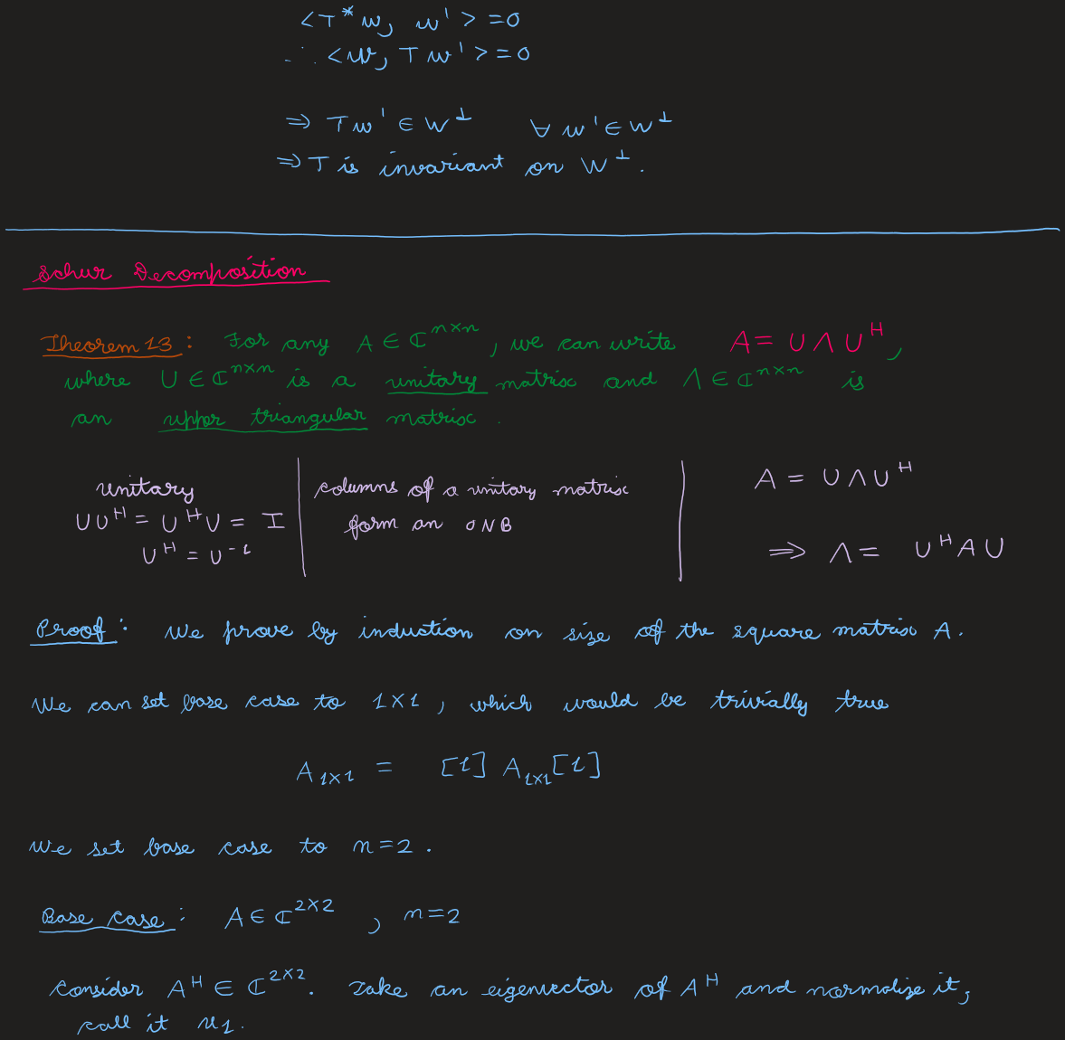
Not all matrices can be diagonalized, but every matrix is similar to an upper triangular matrix. (We need Proposition 6 first.)
Proposition 6
Let \( T \in \Lin(V) \) and \(W\) a subspace of \(V\). Then \(T\) is invariant on \( W^{\perp} \) iff \( T^* \) is invariant on \(W\). (Recall \(T\) is invariant on \( W \subseteq V \) if \( Tw \in W \ \forall\, w \in W \).)
Proof
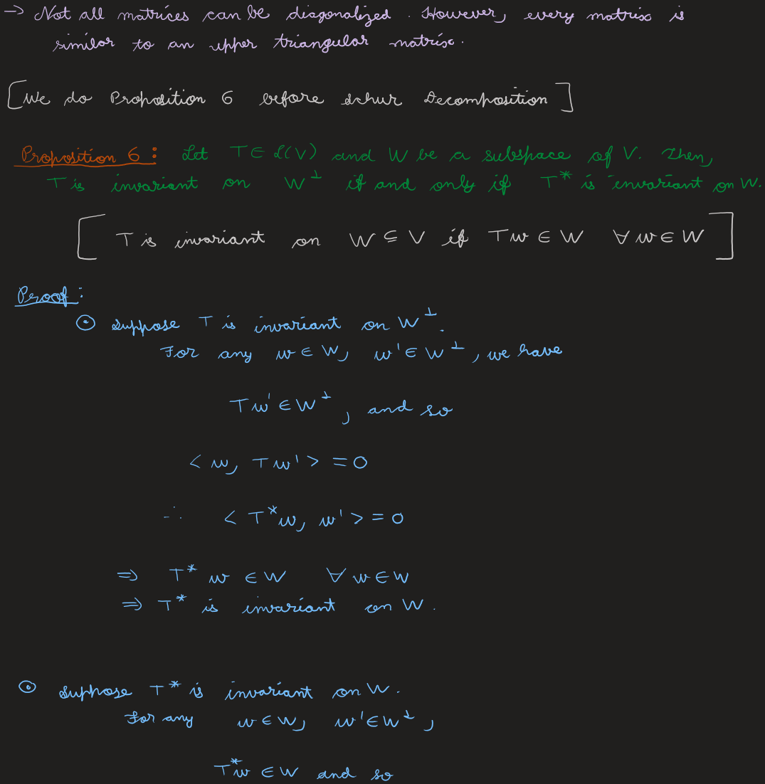
(\( \Rightarrow \)) Suppose \(T\) is invariant on \( W^{\perp} \). For \( w \in W \), \( w' \in W^{\perp} \): \( Tw' \in W^{\perp} \), so \( \langle w, Tw'\rangle = 0 \), giving \( \langle T^*w, w'\rangle = 0 \). Hence \( T^*w \in W \ \forall\, w \in W \), so \( T^* \) is invariant on \(W\).
(\( \Leftarrow \)) Suppose \( T^* \) is invariant on \(W\). For \( w \in W \), \( w' \in W^{\perp} \): \( T^*w \in W \), so \( \langle T^*w, w'\rangle = 0 \), giving \( \langle w, Tw'\rangle = 0 \). Hence \( Tw' \in W^{\perp} \ \forall\, w' \in W^{\perp} \), so \(T\) is invariant on \( W^{\perp} \).
Theorem 13 — Schur Decomposition
For any \( A \in \C^{n\times n} \), we can write \( A = U\Lambda U\herm \), where \( U \in \C^{n\times n} \) is unitary and \( \Lambda \in \C^{n\times n} \) is upper triangular. (Unitary: \( UU\herm = U\herm U = I \), \( U\herm = U^{-1} \), columns form an ONB; equivalently \( \Lambda = U\herm A U \).)
Proof
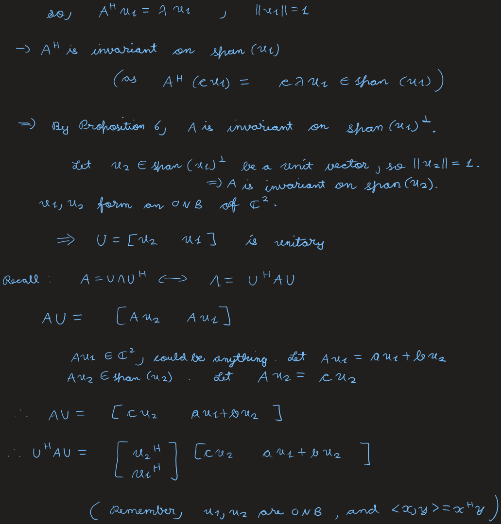
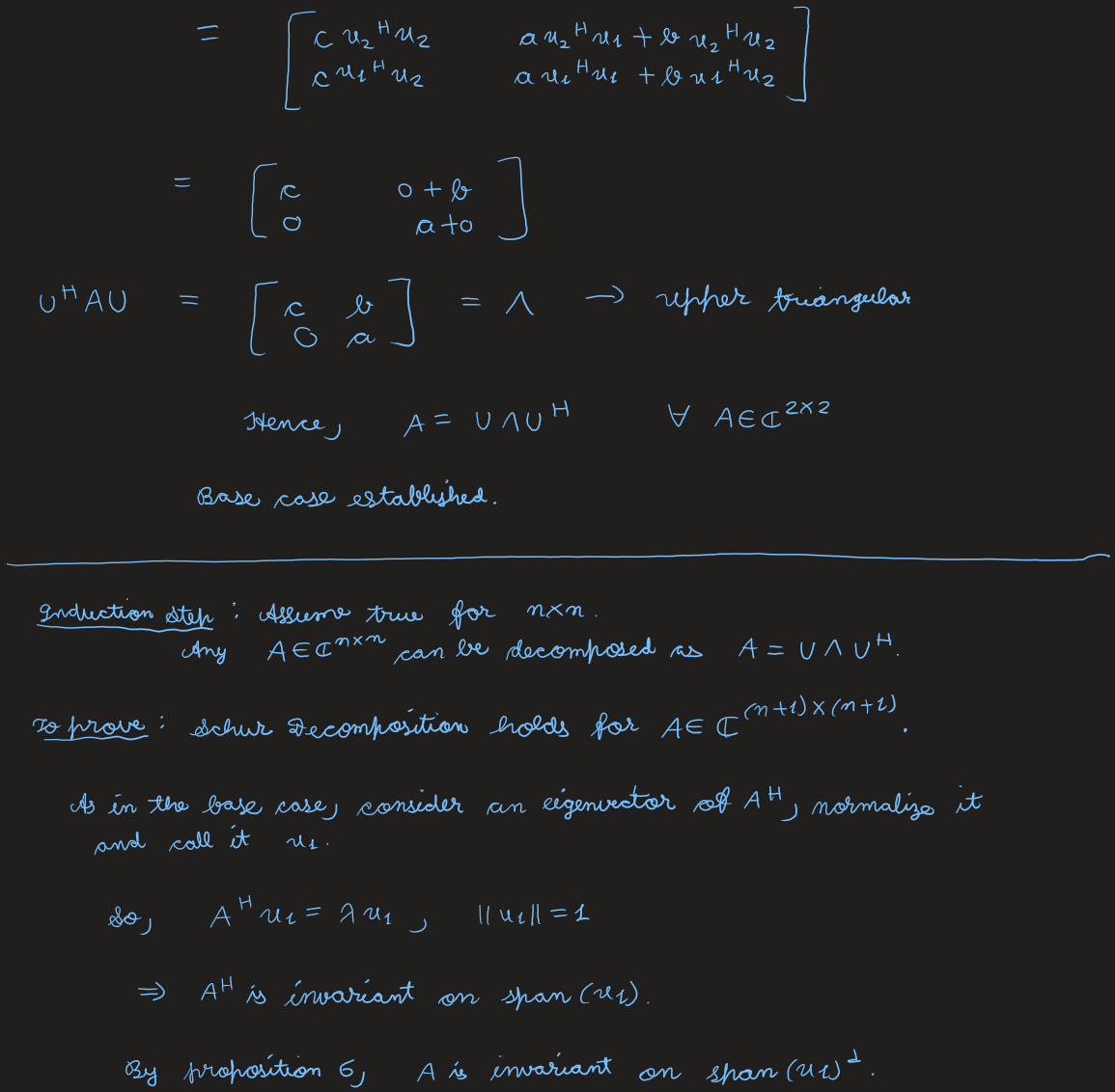
By induction on the size of \(A\). Base case \( n = 2 \), \( A \in \C^{2\times 2} \): take an eigenvector of \( A\herm \), normalized to \( u_1 \) (\( A\herm u_1 = \lambda u_1 \), \( \|u_1\| = 1 \)). Then \( A\herm \) is invariant on \( \operatorname{span}(u_1) \), so by Proposition 6, \(A\) is invariant on \( \operatorname{span}(u_1)^{\perp} \). Pick a unit \( u_2 \in \operatorname{span}(u_1)^{\perp} \); then \( u_1, u_2 \) is an ONB of \( \C^2 \) and \( U = [\,u_2\ u_1\,] \) is unitary. Writing \( Au_1 = a u_1 + b u_2 \), \( Au_2 = c u_2 \) (as \(A\) is invariant on \( \operatorname{span}(u_2) \)), \[ U\herm A U = \begin{bmatrix} u_2\herm \\ u_1\herm \end{bmatrix}\big[\,c u_2 \quad a u_1 + b u_2\,\big] = \begin{bmatrix} c & b \\ 0 & a \end{bmatrix} = \Lambda \quad (\text{upper triangular}), \] using \( \langle x, y\rangle = x\herm y \) and orthonormality. So \( A = U\Lambda U\herm \).
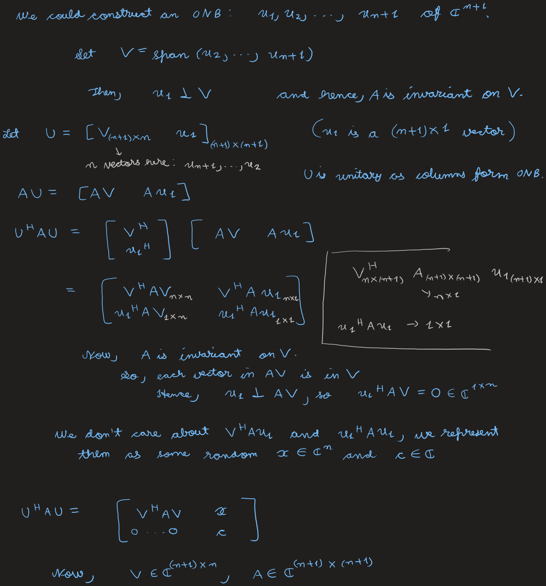
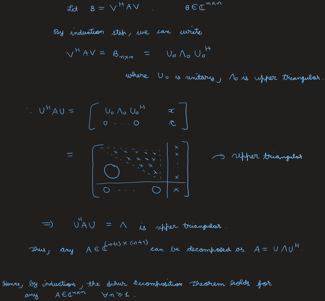
Inductive step. Assume the result for \( n\times n \); take \( A \in \C^{(n+1)\times(n+1)} \). As before, get a unit eigenvector \( u_1 \) of \( A\herm \); then \(A\) is invariant on \( V = \operatorname{span}(u_1)^{\perp} = \operatorname{span}(u_2, \dots, u_{n+1}) \). With \( U = [\,V \mid u_1\,] \) unitary (columns an ONB), \[ U\herm A U = \begin{bmatrix} V\herm A V & x \\ 0 \cdots 0 & c \end{bmatrix}, \] since \( u_1 \perp AV \) gives \( u_1\herm A V = 0 \); \(x\) and \(c\) are arbitrary. Let \( B = V\herm A V \in \C^{n\times n} \); by induction \( B = U_0\Lambda_0 U_0\herm \) with \( \Lambda_0 \) upper triangular. Substituting makes \( U\herm A U \) (after composing the unitaries) upper triangular. Thus \( A = U\Lambda U\herm \), and by induction the Schur decomposition holds for all \( A \in \C^{n\times n} \), \( n \ge 1 \).
Ex 89
Show that the diagonal elements of \( \Lambda \) in the Schur decomposition are exactly the eigenvalues of \(A\).
Solution
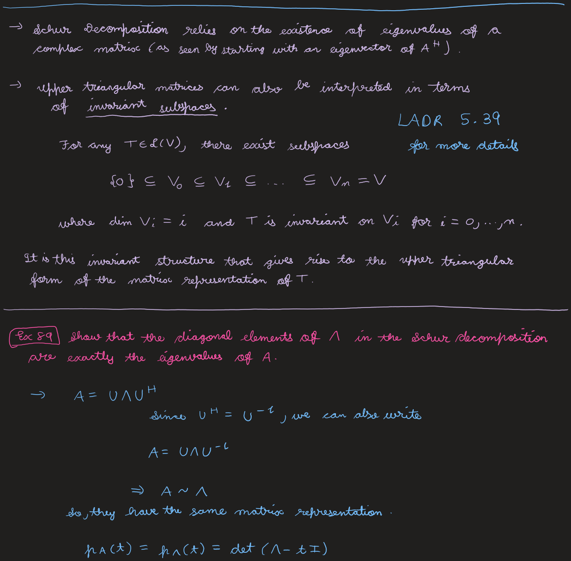
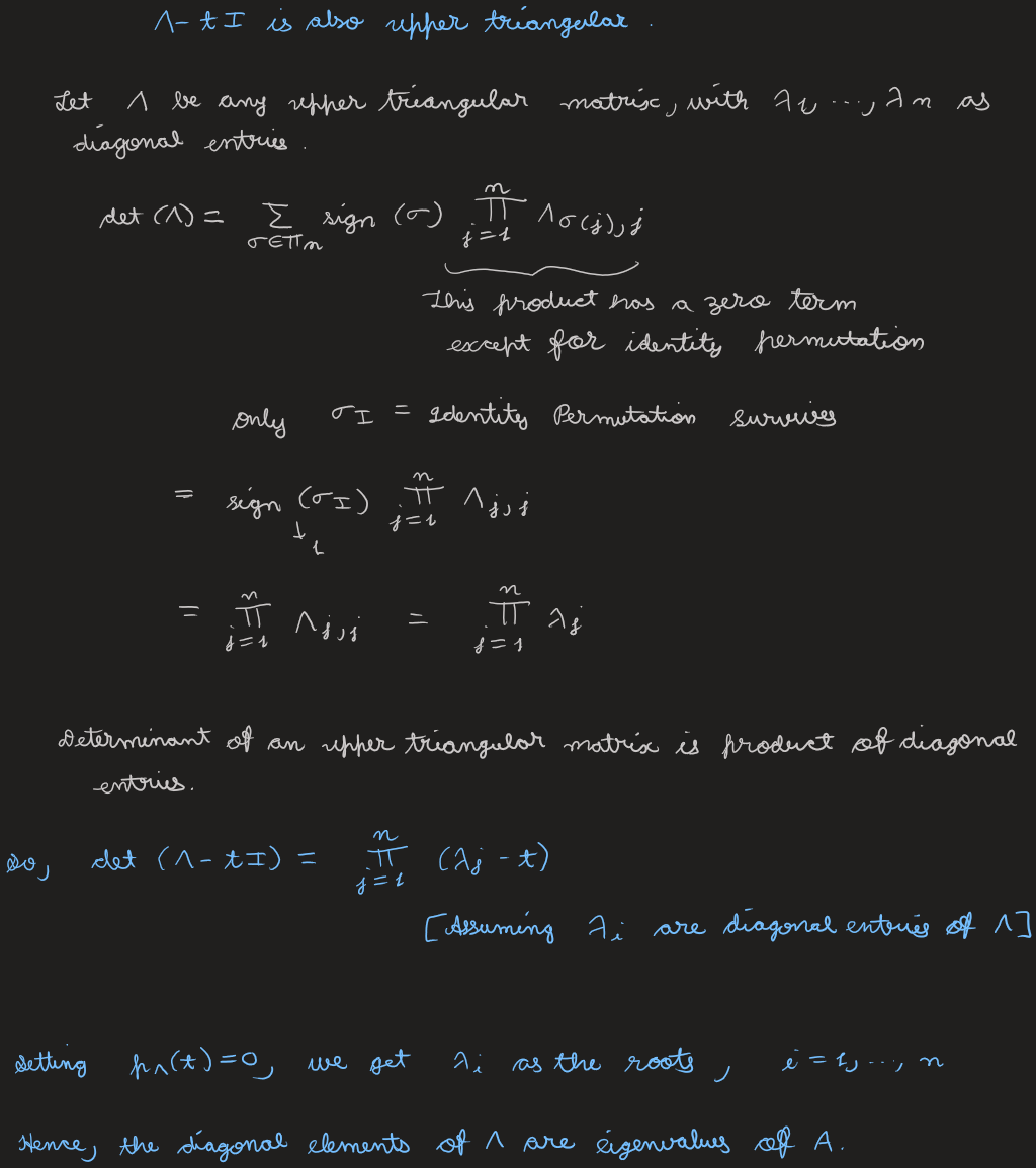
From \( A = U\Lambda U\herm \) with \( U\herm = U^{-1} \), \( \Lambda = U\herm A U \), so \( A \sim \Lambda \) and \( f_A(t) = f_\Lambda(t) = \det(\Lambda - tI) \). For an upper triangular matrix \( \Lambda \) with diagonal \( \lambda_1, \dots, \lambda_n \), the Leibniz expansion leaves only the identity permutation, so \( \det(\Lambda) = \prod_{i=1}^{n}\lambda_i \) (determinant of an upper triangular matrix is the product of its diagonal). Hence \( \det(\Lambda - tI) = \prod_{i=1}^{n}(\lambda_i - t) \), whose roots are \( \lambda_1, \dots, \lambda_n \). So the diagonal of \( \Lambda \) gives the eigenvalues of \(A\).
Remark
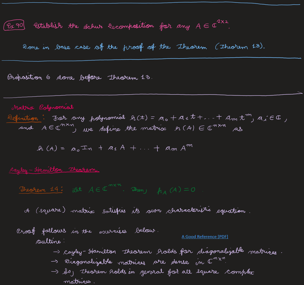
The Schur decomposition relies on the existence of eigenvectors of a complex matrix (start from an eigenvector of \( A\herm \)). Upper triangular matrices also correspond to a flag of invariant subspaces (LADR 5.39): for \( T \in \Lin(V) \) there are \( \{0\} \subseteq V_1 \subseteq \dots \subseteq V_n = V \) with \( \dim V_i = i \) and \(T\) invariant on each \( V_i \) — this invariant structure is what yields the upper triangular representation. (Ex 90 asks to establish the Schur decomposition for \( A \in \C^{2\times 2} \) — the base case of the induction above.)
View original handwritten scans — Schur decomposition, Ex 89–90 (pages 22–30)
Matrix Polynomials & Cayley–Hamilton
Definition 44 — Matrix polynomial
For a polynomial \( p(z) = a_0 + a_1 z + \dots + a_m z^m \) (\( a_i \in \C \)) and \( A \in \C^{n\times n} \), define \( p(A) = a_0 I + a_1 A + \dots + a_m A^m \in \C^{n\times n} \).
Theorem 14 — Cayley–Hamilton
Every square matrix satisfies its own characteristic equation: for \( A \in \C^{n\times n} \), \( f_A(A) = 0 \).
Ex 91
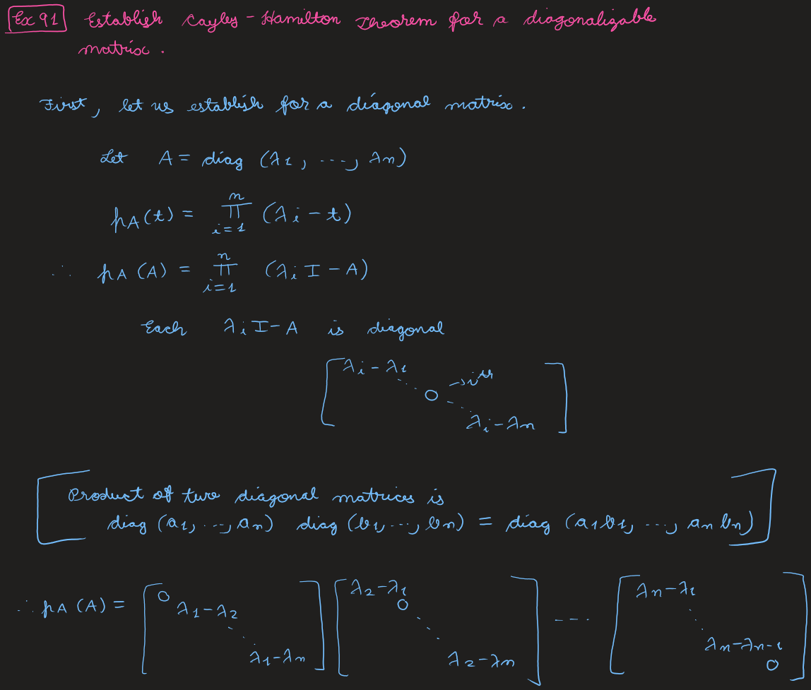
Establish the Cayley–Hamilton theorem for a diagonalizable matrix.
Solution
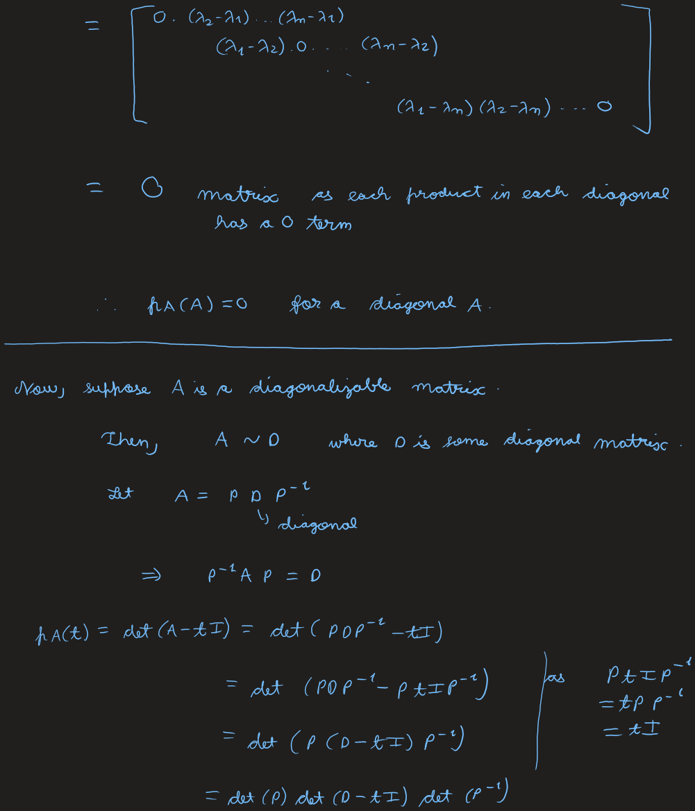
Diagonal case. For \( A = \diag(\lambda_1, \dots, \lambda_n) \), \( f_A(t) = \prod_{i=1}^{n}(\lambda_i - t) \), so \( f_A(A) = \prod_{i=1}^{n}(\lambda_i I - A) \). Each \( \lambda_i I - A = \diag(\lambda_i - \lambda_1, \dots, \lambda_i - \lambda_n) \) is diagonal with a \(0\) in the \(i\)-th slot. Since the product of diagonal matrices multiplies entrywise, the \(j\)-th diagonal entry of \( \prod_i(\lambda_i I - A) \) contains the factor \( (\lambda_j - \lambda_j) = 0 \). Hence \( f_A(A) = O \) for diagonal \(A\).
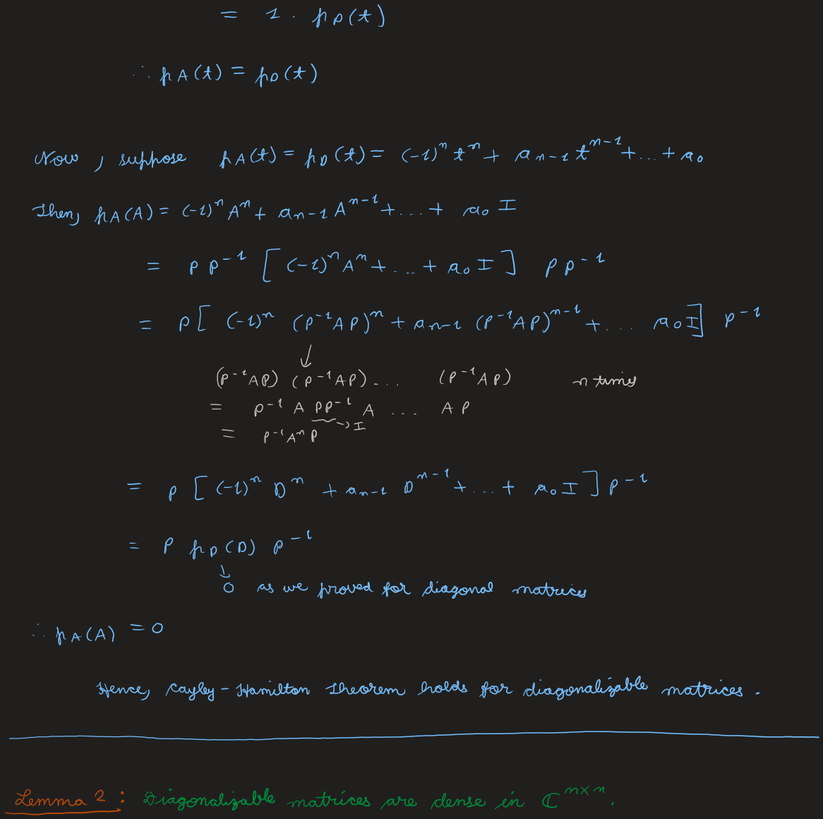
Diagonalizable case. If \( A = PDP^{-1} \) with \(D\) diagonal, then \( f_A(t) = f_D(t) \) (similar matrices). Writing \( f_A(t) = (-1)^n t^n + a_{n-1}t^{n-1} + \dots + a_0 \), \[\begin{aligned} f_A(A) &= (-1)^n A^n + \dots + a_0 I \\ &= P\big[(-1)^n(P^{-1}AP)^n + \dots + a_0 I\big]P^{-1} \\ &= P\,f_D(D)\,P^{-1}, \end{aligned}\] using \( (P^{-1}AP)^m = P^{-1}A^m P \). Since \( f_D(D) = 0 \), \( f_A(A) = 0 \). Hence Cayley–Hamilton holds for diagonalizable matrices.
Lemma 2
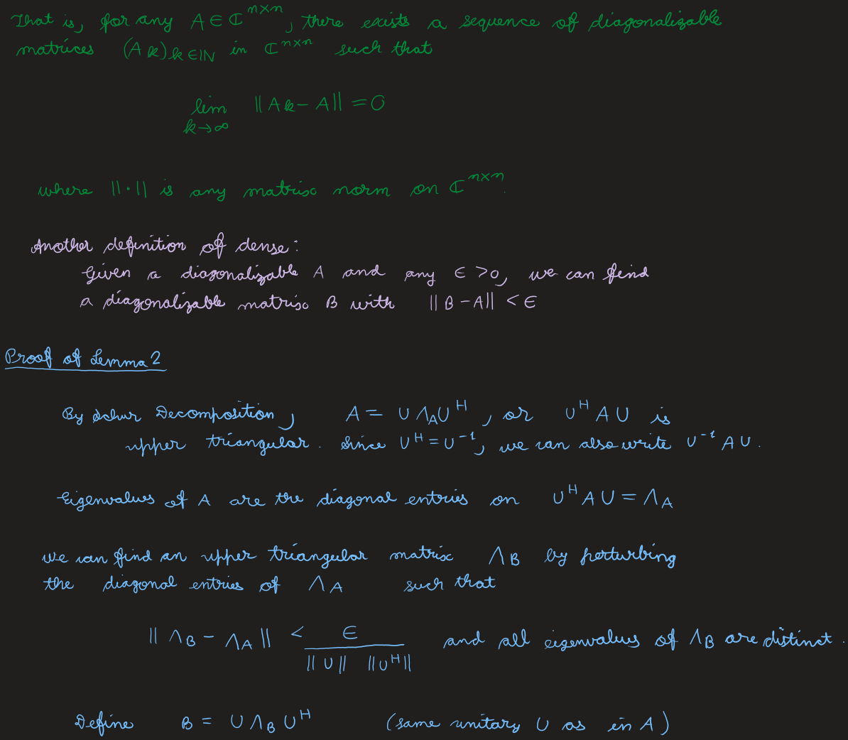
Diagonalizable matrices are dense in \( \C^{n\times n} \): for any \( A \in \C^{n\times n} \) there is a sequence of diagonalizable \( (A_k)_{k\in\N} \) with \( \lim_{k\to\infty}\|A_k - A\| = 0 \) (any matrix norm). Equivalently, given any \(A\) and \( \varepsilon > 0 \), there is a diagonalizable \(B\) with \( \|B - A\| < \varepsilon \).
Proof
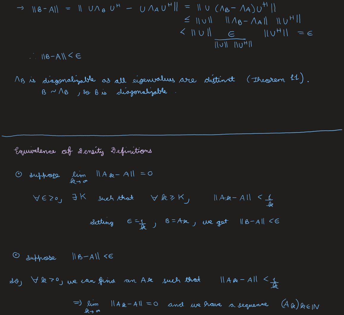
By Schur, \( A = U\Lambda_A U\herm \) with \( \Lambda_A = U\herm A U \) upper triangular; the eigenvalues of \(A\) are its diagonal entries. Perturb the diagonal of \( \Lambda_A \) to an upper triangular \( \Lambda_B \) with all eigenvalues distinct and \( \|\Lambda_B - \Lambda_A\| < \dfrac{\varepsilon}{\|U\|\,\|U\herm\|} \). Define \( B = U\Lambda_B U\herm \). Then \[ \|B - A\| = \|U(\Lambda_B - \Lambda_A)U\herm\| \le \|U\|\,\|\Lambda_B - \Lambda_A\|\,\|U\herm\| < \varepsilon. \] \( \Lambda_B \) has distinct eigenvalues, hence is diagonalizable (Theorem 11), and \( B \sim \Lambda_B \), so \(B\) is diagonalizable.
Equivalence of the density definitions. If \( \lim_k\|A_k - A\| = 0 \), then for each \(k\) eventually \( \|A_k - A\| < \tfrac1k \); setting \( \varepsilon = \tfrac1k \), \( B = A_k \) gives \( \|B - A\| < \varepsilon \). Conversely, choosing \( A_k \) with \( \|A_k - A\| < \tfrac1k \) for each \(k\) yields \( \lim_k\|A_k - A\| = 0 \).
Cayley–Hamilton for all matrices
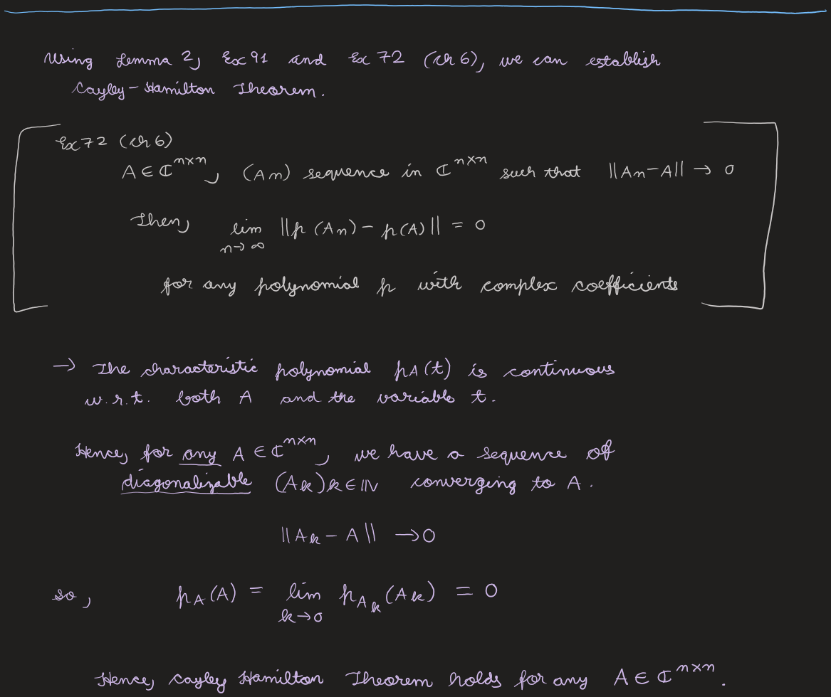
Using Lemma 2, Ex 91, and Ex 72 of Ch. 6 (if \( \|A_n - A\| \to 0 \) then \( \|p(A_n) - p(A)\| \to 0 \) for any polynomial \(p\)): the characteristic polynomial \( f_A(t) \) is continuous in both \(A\) and \(t\). For any \( A \in \C^{n\times n} \) take diagonalizable \( A_k \to A \). Since \( f_{A_k}(A_k) = 0 \) (Ex 91) and everything is continuous, \[ f_A(A) = \lim_{k\to\infty} f_{A_k}(A_k) = 0. \] Hence the Cayley–Hamilton theorem holds for any \( A \in \C^{n\times n} \).
View original handwritten scans — Matrix polynomials & Cayley–Hamilton (pages 30–36)