Chapter 5 — Transforms on Inner Product Spaces
Linear Algebra and its Applications · IISc 2024 · typeset reproduction
Orthogonal Projector
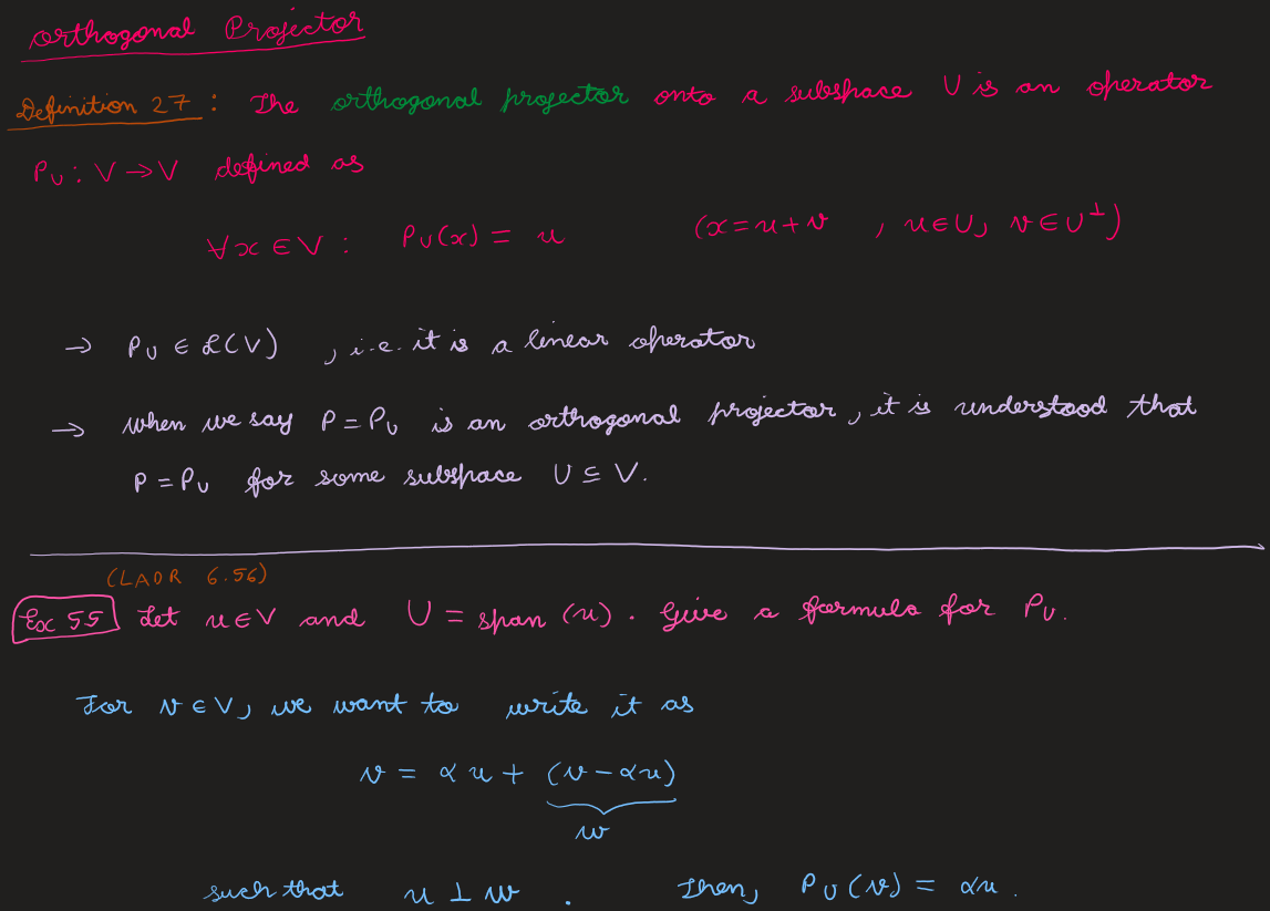
Definition 27 — Orthogonal projector
The orthogonal projector onto a subspace \( U \) is an operator \( P_U : V \to V \) defined as \[ \forall\, x \in V : \quad P_U(x) = u \qquad (x = u + v,\ u \in U,\ v \in U^{\perp}). \]
- \( P_U \in \Lin(V) \), i.e. it is a linear operator.
- When we say \( P = P_U \) is an orthogonal projector, it is understood that \( P = P_U \) for some subspace \( U \subseteq V \).
Ex 55 — LADR 6.56
Let \( u \in V \) and \( U = \operatorname{span}(u) \). Give a formula for \( P_U \).
Solution
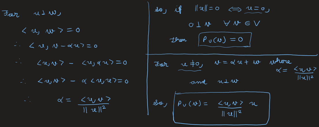
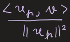
For \( v \in V \), write \( v = \alpha u + (v - \alpha u) \) with \( w = v - \alpha u \) such that \( u \perp w \); then \( P_U(v) = \alpha u \). From \( \langle u, w\rangle = 0 \): \[ \langle u, v - \alpha u\rangle = 0 \implies \langle u, v\rangle - \alpha\langle u, u\rangle = 0 \implies \alpha = \frac{\langle u, v\rangle}{\|u\|^2}. \] So if \( \|u\| = 0 \iff u = 0 \) (and \( 0 \perp v \ \forall\, v \in V \)), then \( P_U(v) = 0 \). For \( u \neq 0 \), \[ \boxed{\ P_U(v) = \frac{\langle u, v\rangle}{\|u\|^2}\, u\ }. \]
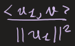
If \( u_1, \dots, u_n \) is an orthogonal basis for \( V \), then we can write \[ P_U(v) = \frac{\langle u_1, v\rangle}{\|u_1\|^2}\, u_1 + \dots + \frac{\langle u_n, v\rangle}{\|u_n\|^2}\, u_n \qquad \text{for } v \in V. \]
View original handwritten scans — orthogonal projector, Def 27 & Ex 55 (pages 1–14; the projection formula was fragmented across a layout grid, shown side-by-side)




Properties of the Orthogonal Projector
Ex 56 — LADR 6.57, 6.61
Let \( P = P_U \) be an orthogonal projector on \( V \). Show that:
- \( P^2 = P \);
- \( \Range(P) = U \) and \( \Null(P) = U^{\perp} \);
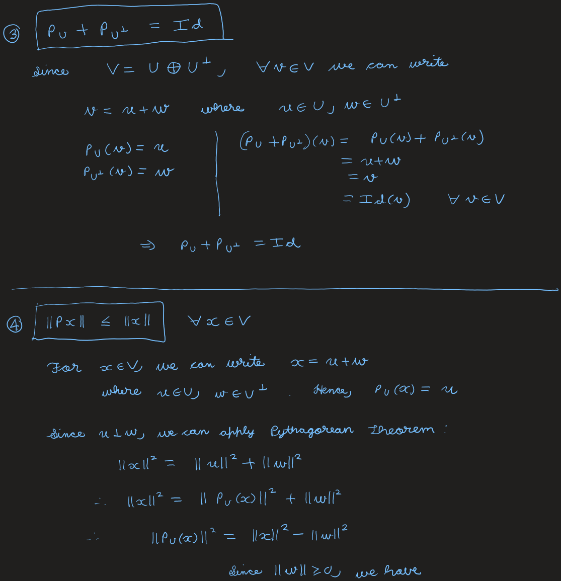
- \( P_U + P_{U^{\perp}} = \mathrm{Id} \);
- \( \|Px\| \le \|x\| \ \forall\, x \in V \);
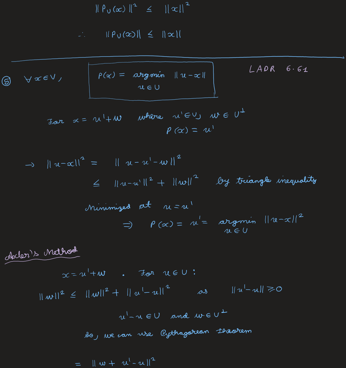
- \( \forall\, x \in V \), \( P(x) = \displaystyle\operatorname*{arg\,min}_{u \in U} \|u - x\| \) — i.e. \( P(x) \) is the (unique) point in \( U \) that is "closest" to \( x \).
Solution
Throughout, write \( v = u + w \) with \( u \in U \), \( w \in U^{\perp} \), so \( P_U(v) = u \).
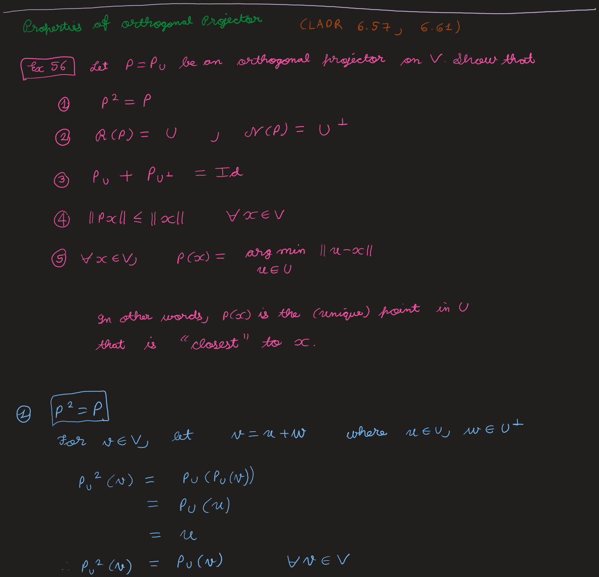
(1) \( P^2 = P \). \( P_U^2(v) = P_U(P_U(v)) = P_U(u) = u = P_U(v) \ \forall\, v \in V \), so \( P^2 = P \).
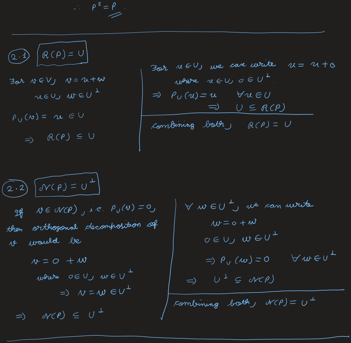
(2) \( \Range(P) = U \), \( \Null(P) = U^{\perp} \). \( P_U(v) = u \in U \Rightarrow \Range(P) \subseteq U \); and for \( u \in U \), \( u = u + 0 \Rightarrow P_U(u) = u \Rightarrow U \subseteq \Range(P) \). So \( \Range(P) = U \). If \( P_U(v) = 0 \), the decomposition is \( v = 0 + w \Rightarrow v = w \in U^{\perp} \Rightarrow \Null(P) \subseteq U^{\perp} \); and for \( w \in U^{\perp} \), \( w = 0 + w \Rightarrow P_U(w) = 0 \Rightarrow U^{\perp} \subseteq \Null(P) \). So \( \Null(P) = U^{\perp} \).
(3) \( P_U + P_{U^{\perp}} = \mathrm{Id} \). Since \( V = U \oplus U^{\perp} \), \( v = u + w \) gives \( P_U(v) = u \), \( P_{U^{\perp}}(v) = w \), so \( (P_U + P_{U^{\perp}})(v) = u + w = v = \mathrm{Id}(v) \ \forall\, v \).
(4) \( \|Px\| \le \|x\| \). For \( x = u + w \), \( P_U(x) = u \) and \( u \perp w \), so by the Pythagorean theorem \( \|x\|^2 = \|u\|^2 + \|w\|^2 = \|P_U(x)\|^2 + \|w\|^2 \). Hence \( \|P_U(x)\|^2 = \|x\|^2 - \|w\|^2 \le \|x\|^2 \), i.e. \( \|P_U(x)\| \le \|x\| \).
(5) Closest point (Axler's method). Write \( x = u' + w \) with \( u' \in U \), \( w \in U^{\perp} \), so \( P(x) = u' \). For any \( u \in U \), \( u' - u \in U \) and \( w \in U^{\perp} \) are orthogonal, so by the Pythagorean theorem \[ \|u - x\|^2 = \|(u' - u) + w\|^2 = \|u' - u\|^2 + \|w\|^2 \ge \|w\|^2, \] with equality iff \( u = u' \). Hence \( P(x) = u' = \operatorname*{arg\,min}_{u \in U}\|u - x\|^2 \).
Ex 57
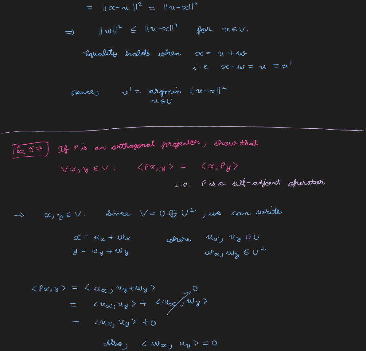
If \( P \) is an orthogonal projector, show that \( \forall\, x, y \in V : \langle Px, y\rangle = \langle x, Py\rangle \), i.e. \( P \) is a self-adjoint operator.
Solution
Since \( V = U \oplus U^{\perp} \), write \( x = u_x + w_x \), \( y = u_y + w_y \) with \( u_x, u_y \in U \), \( w_x, w_y \in U^{\perp} \). Then \[\begin{aligned} \langle Px, y\rangle &= \langle u_x, u_y + w_y\rangle \\ &= \langle u_x, u_y\rangle + \underbrace{\langle u_x, w_y\rangle}_{0} = \langle u_x, u_y\rangle + \underbrace{\langle w_x, u_y\rangle}_{0} \\ &= \langle u_x + w_x, u_y\rangle = \langle x, Py\rangle. \end{aligned}\]
View original handwritten scans — properties of the orthogonal projector, Ex 56–57 (pages 15–20)
The Adjoint
The definition of the adjoint is motivated by the following result.
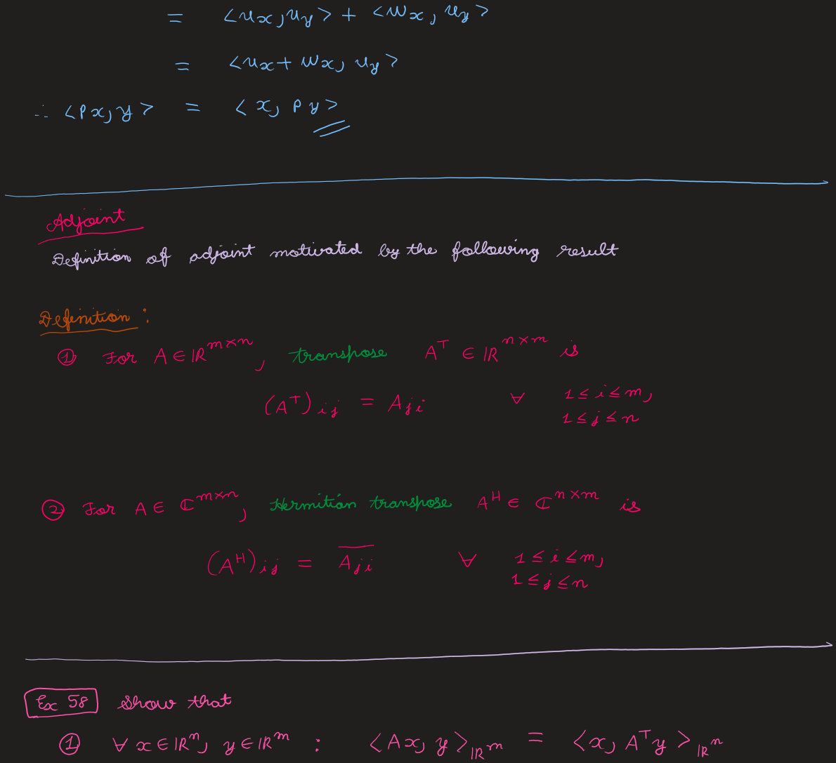
Definition — Transpose & Hermitian transpose
- For \( A \in \R^{m\times n} \), the transpose \( A\T \in \R^{n\times m} \) is \( (A\T)_{ij} = A_{ji} \).
- For \( A \in \C^{m\times n} \), the Hermitian transpose \( A\herm \in \C^{n\times m} \) is \( (A\herm)_{ij} = \overline{A_{ji}} \).
Ex 58
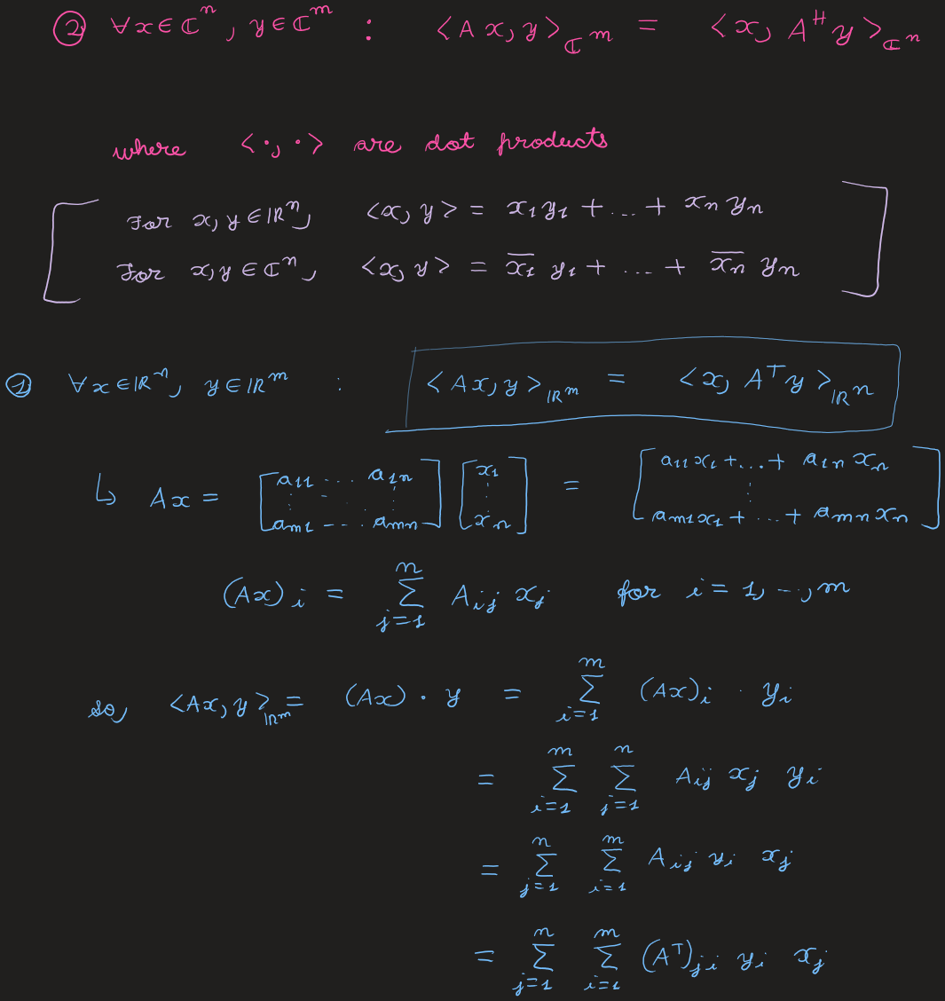
Show that (with \( \langle\cdot,\cdot\rangle \) the dot products):
- \( \forall\, x \in \R^n,\ y \in \R^m : \langle Ax, y\rangle_{\R^m} = \langle x, A\T y\rangle_{\R^n} \);
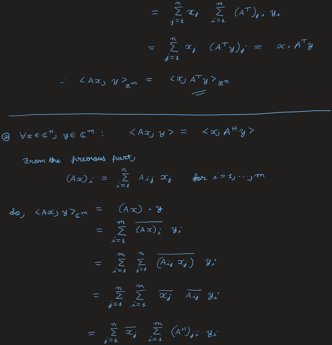
- \( \forall\, x \in \C^n,\ y \in \C^m : \langle Ax, y\rangle_{\C^m} = \langle x, A\herm y\rangle_{\C^n} \).
Solution
With \( (Ax)_i = \sum_{j=1}^{n} A_{ij} x_j \) for \( i = 1, \dots, m \):
(1) Real case. \[\begin{aligned} \langle Ax, y\rangle_{\R^m} &= \sum_{i=1}^{m} (Ax)_i\, y_i = \sum_{i=1}^{m}\sum_{j=1}^{n} A_{ij} x_j y_i \\ &= \sum_{j=1}^{n} x_j \sum_{i=1}^{m} (A\T)_{ji}\, y_i \\ &= \sum_{j=1}^{n} x_j\, (A\T y)_j = \langle x, A\T y\rangle_{\R^n}. \end{aligned}\]
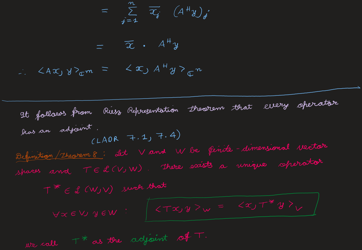
(2) Complex case. \[\begin{aligned} \langle Ax, y\rangle_{\C^m} &= \sum_{i=1}^{m} \overline{(Ax)_i}\, y_i = \sum_{i=1}^{m}\sum_{j=1}^{n} \overline{x_j}\,\overline{A_{ij}}\, y_i \\ &= \sum_{j=1}^{n} \overline{x_j} \sum_{i=1}^{m} (A\herm)_{ji}\, y_i \\ &= \sum_{j=1}^{n} \overline{x_j}\,(A\herm y)_j = \langle x, A\herm y\rangle_{\C^n}. \end{aligned}\]
It follows from the Riesz Representation Theorem that every operator has an adjoint.
Definition / Theorem 8 — Adjoint (LADR 7.1, 7.4)
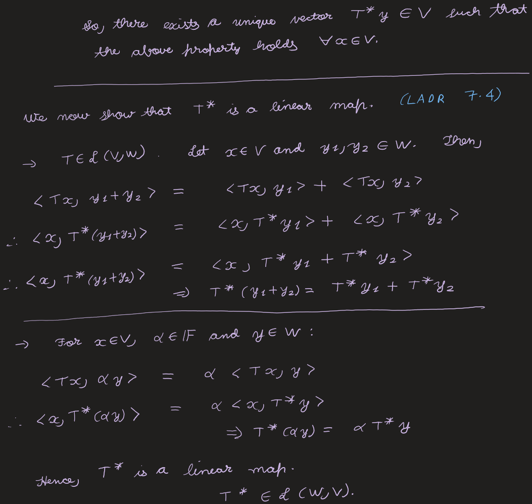
Let \( V \) and \( W \) be finite-dimensional vector spaces and \( T \in \Lin(V, W) \). There exists a unique operator \( T^* \in \Lin(W, V) \) such that \[ \forall\, x \in V,\ y \in W : \quad \langle Tx, y\rangle_W = \langle x, T^* y\rangle_V. \] We call \( T^* \) the adjoint of \( T \).
Proof
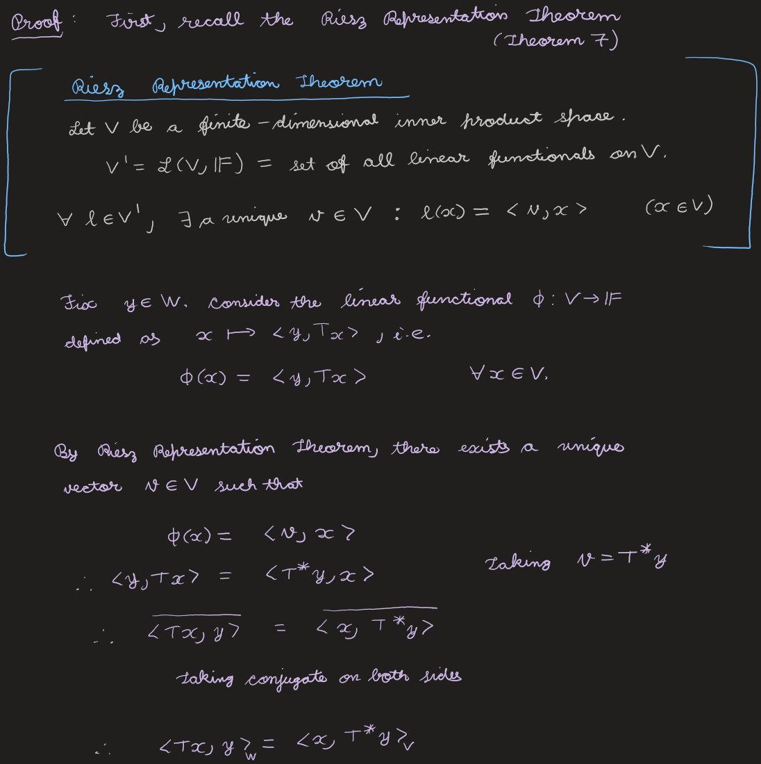
Recall the Riesz Representation Theorem (Theorem 7): for a finite-dimensional inner product space \( V \), every linear functional \( \ell \in V' \) is \( \ell(x) = \langle v, x\rangle \) for a unique \( v \in V \).
Fix \( y \in W \) and consider the linear functional \( \phi : V \to \F \), \( \phi(x) = \langle y, Tx\rangle \). By Riesz, there is a unique \( v \in V \) with \( \phi(x) = \langle v, x\rangle \); write \( v = T^* y \). Then \( \langle y, Tx\rangle = \langle T^* y, x\rangle \); taking conjugates, \( \langle Tx, y\rangle_W = \langle x, T^* y\rangle_V \), and \( T^* y \) is unique.
\( T^* \) is linear. For \( y_1, y_2 \in W \): \( \langle Tx, y_1 + y_2\rangle = \langle Tx, y_1\rangle + \langle Tx, y_2\rangle \) gives \( \langle x, T^*(y_1 + y_2)\rangle = \langle x, T^* y_1 + T^* y_2\rangle \ \forall\, x \), so \( T^*(y_1 + y_2) = T^* y_1 + T^* y_2 \). For \( \alpha \in \F \): \( \langle Tx, \alpha y\rangle = \alpha\langle Tx, y\rangle \) gives \( \langle x, T^*(\alpha y)\rangle = \alpha\langle x, T^* y\rangle \), so \( T^*(\alpha y) = \alpha T^* y \). Hence \( T^* \in \Lin(W, V) \).
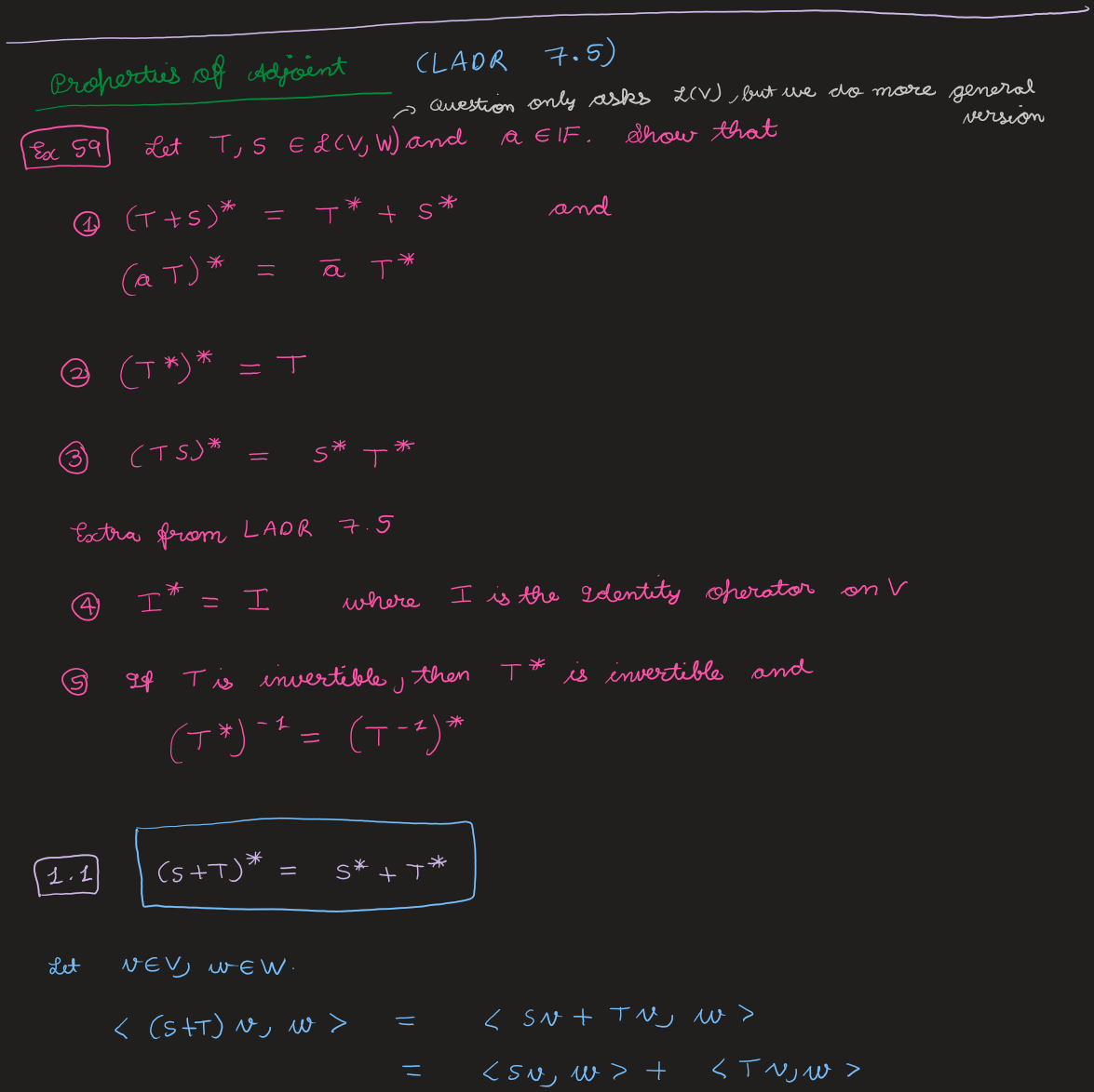
Ex 59 — Properties of the adjoint (LADR 7.5)
Let \( T, S \in \Lin(V) \) and \( a \in \F \). Show that
- \( (T + S)^* = T^* + S^* \) and \( (aT)^* = \bar a\, T^* \);
- \( (T^*)^* = T \);
- \( (TS)^* = S^* T^* \);
- \( I^* = I \) (\( I \) the identity operator on \( V \));
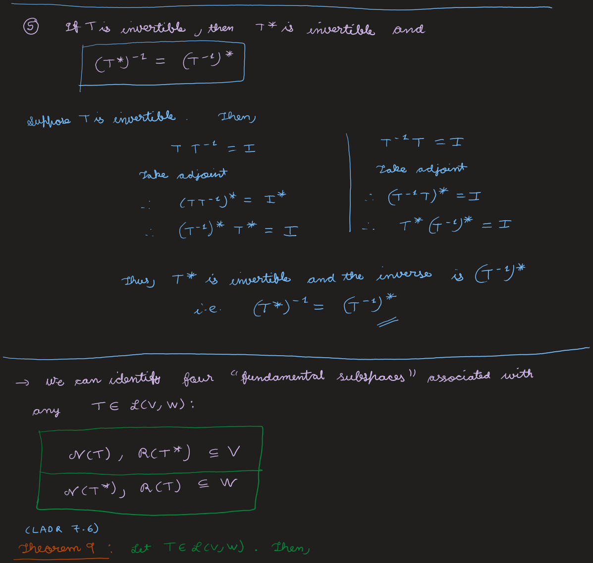
- if \( T \) is invertible, then \( T^* \) is invertible and \( (T^*)^{-1} = (T^{-1})^* \).
Solution
Each identity follows by moving operators across \( \langle\cdot,\cdot\rangle \) and using uniqueness of the adjoint.
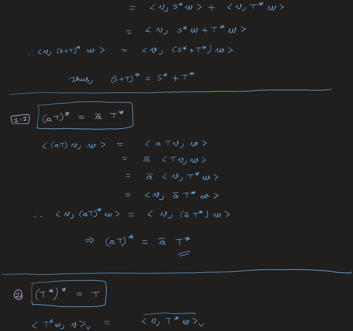
(1) \( \langle (S+T)v, w\rangle = \langle Sv, w\rangle + \langle Tv, w\rangle = \langle v, (S^* + T^*)w\rangle \Rightarrow (S+T)^* = S^* + T^* \). And \( \langle (aT)v, w\rangle = \bar a\langle Tv, w\rangle = \langle v, \bar a T^* w\rangle \Rightarrow (aT)^* = \bar a\, T^* \).
(2) \( \langle T^* w, v\rangle = \overline{\langle v, T^* w\rangle} = \overline{\langle Tv, w\rangle} = \langle w, Tv\rangle \), and \( \langle T^* w, v\rangle = \langle w, (T^*)^* v\rangle \), so \( (T^*)^* = T \).
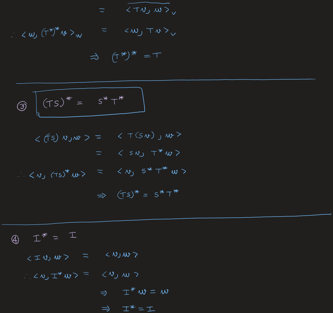
(3) \( \langle (TS)v, w\rangle = \langle T(Sv), w\rangle = \langle Sv, T^* w\rangle = \langle v, S^* T^* w\rangle \Rightarrow (TS)^* = S^* T^* \).
(4) \( \langle Iv, w\rangle = \langle v, w\rangle \Rightarrow \langle v, I^* w\rangle = \langle v, w\rangle \Rightarrow I^* = I \).
(5) From \( TT^{-1} = I \), taking adjoints, \( (T^{-1})^* T^* = I \); from \( T^{-1}T = I \), \( T^*(T^{-1})^* = I \). So \( T^* \) is invertible with \( (T^*)^{-1} = (T^{-1})^* \).
View original handwritten scans — transpose/Hermitian transpose, Ex 58, the adjoint (Thm 8) & Ex 59 (pages 20–29)
The Four Fundamental Subspaces
We can identify four "fundamental subspaces" associated with any \( T \in \Lin(V, W) \): \( \Null(T),\ \Range(T^*) \subseteq V \) and \( \Null(T^*),\ \Range(T) \subseteq W \).
Theorem 9 — LADR 7.6
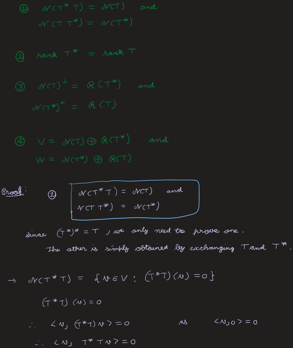
Let \( T \in \Lin(V, W) \). Then
- \( \Null(T^*T) = \Null(T) \) and \( \Null(TT^*) = \Null(T^*) \);
- \( \rank T^* = \rank T \);
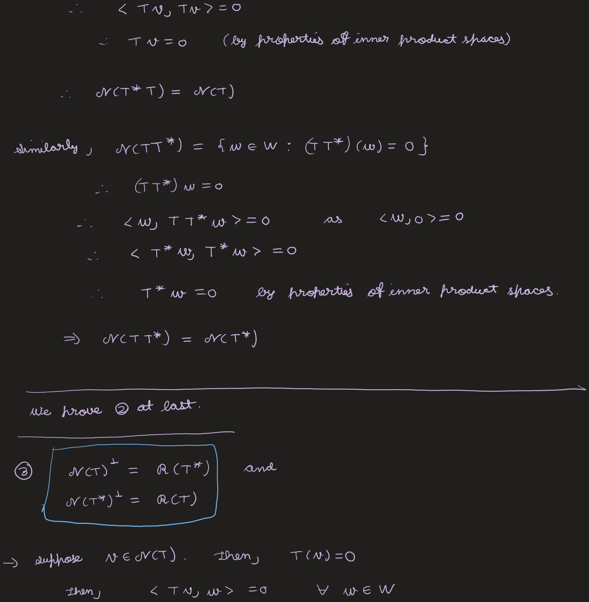
- \( \Null(T)^{\perp} = \Range(T^*) \) and \( \Null(T^*)^{\perp} = \Range(T) \);
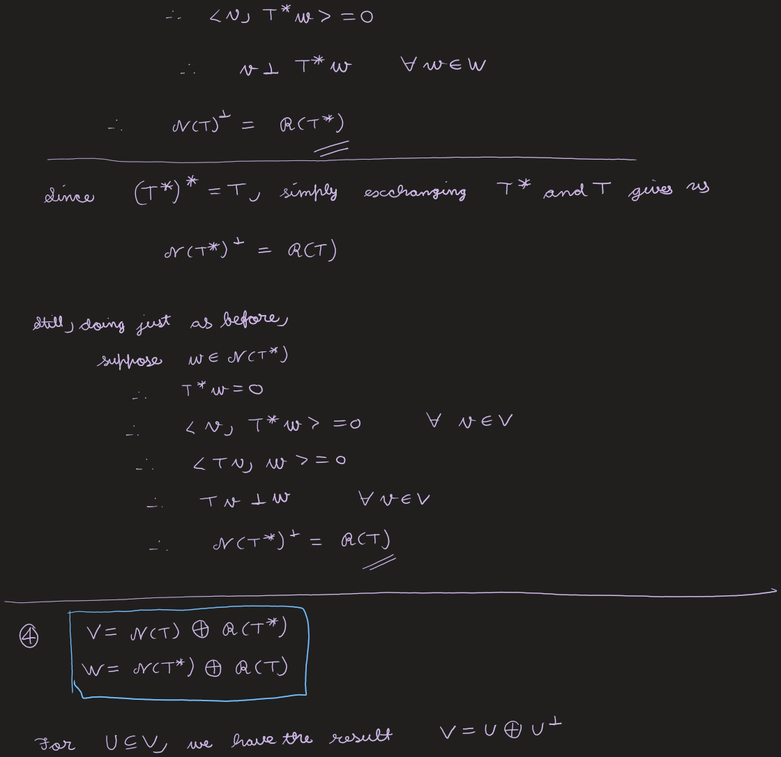
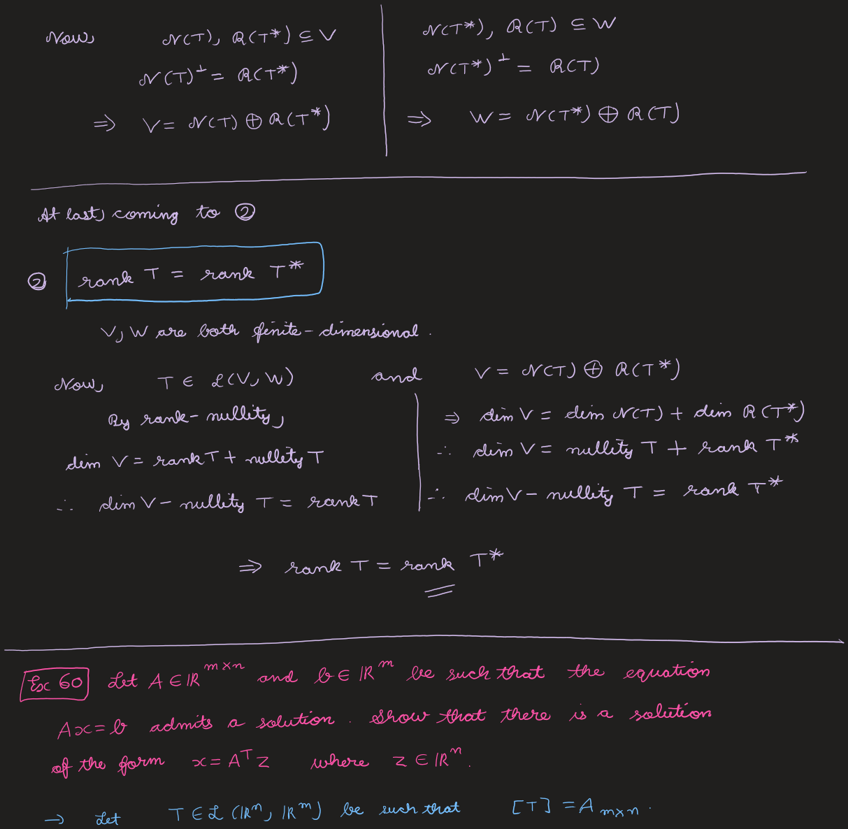
- \( V = \Null(T) \oplus \Range(T^*) \) and \( W = \Null(T^*) \oplus \Range(T) \).
Proof
(1) Since \( (T^*)^* = T \), we only prove one (the other follows by exchanging \( T \leftrightarrow T^* \)). If \( (T^*T)v = 0 \), then \( \langle v, T^*Tv\rangle = 0 \), i.e. \( \langle Tv, Tv\rangle = 0 \), so \( Tv = 0 \). Hence \( \Null(T^*T) = \Null(T) \); similarly \( \Null(TT^*) = \Null(T^*) \).
(3) Suppose \( v \in \Null(T) \), so \( Tv = 0 \) and \( \langle Tv, w\rangle = 0 \ \forall\, w \), i.e. \( \langle v, T^*w\rangle = 0 \), so \( v \perp T^*w \). Hence \( \Null(T)^{\perp} = \Range(T^*) \); exchanging \( T \leftrightarrow T^* \) gives \( \Null(T^*)^{\perp} = \Range(T) \).
(4) For any subspace \( U \subseteq V \) we have \( V = U \oplus U^{\perp} \). With \( \Null(T)^{\perp} = \Range(T^*) \), \( V = \Null(T) \oplus \Range(T^*) \); and \( W = \Null(T^*) \oplus \Range(T) \).
(2) By rank–nullity, \( \dim V = \rank T + \nullity T \). From \( V = \Null(T) \oplus \Range(T^*) \), \( \dim V = \nullity T + \rank T^* \). Equating, \( \rank T = \rank T^* \).
Ex 60
Let \( A \in \R^{m\times n} \) and \( b \in \R^m \) be such that \( Ax = b \) admits a solution. Show that there is a solution of the form \( x = A\T z \) where \( z \in \R^m \).
Solution
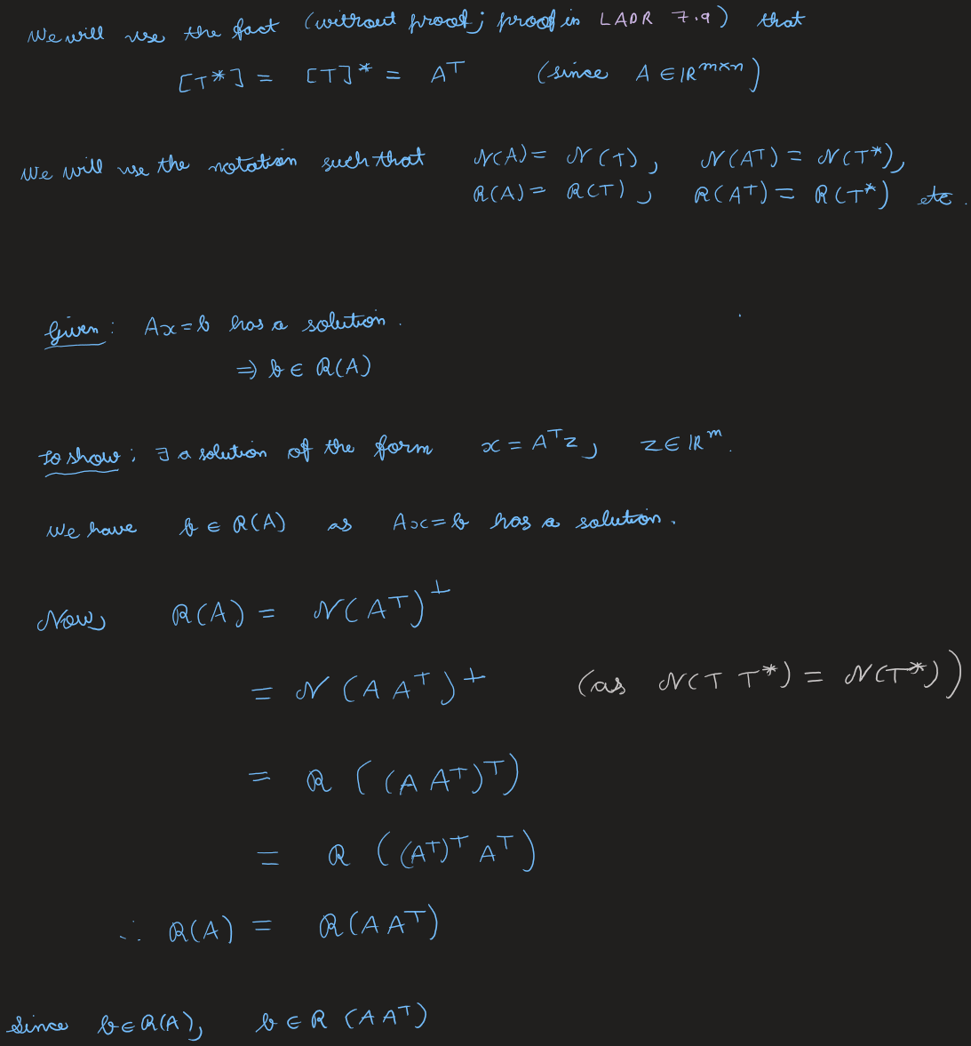
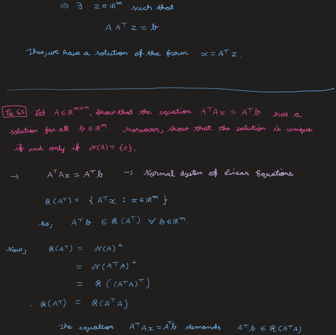
Let \( T \) with \( [T] = A \), so \( [T^*] = A\T \) (since \( A \in \R^{m\times n} \); used without proof, LADR 7.9), and \( \Null(A) = \Null(T) \), \( \Range(A) = \Range(T) \), etc. Given \( Ax = b \) has a solution, \( b \in \Range(A) \). Now \[\begin{aligned} \Range(A) &= \Null(A\T)^{\perp} = \Null(AA\T)^{\perp} \\ &= \Range\big((AA\T)\T\big) = \Range\big((A\T)\T A\T\big) = \Range(AA\T), \end{aligned}\] using \( \Null(TT^*) = \Null(T^*) \) and \( (AA\T)\T = AA\T \). Since \( b \in \Range(A) = \Range(AA\T) \), there exists \( z \in \R^m \) with \( AA\T z = b \), i.e. \( A(A\T z) = b \). Thus \( x = A\T z \) is a solution.
Ex 61 — Normal equations
Let \( A \in \R^{m\times n} \). Show that \( A\T A x = A\T b \) has a solution for all \( b \in \R^m \). Moreover, show that the solution is unique if and only if \( \Null(A) = \{0\} \).
Solution
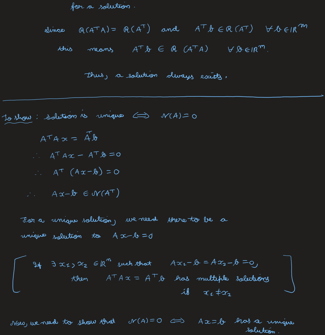
Existence. \( A\T b \in \Range(A\T) \) for all \( b \). And \[\begin{aligned} \Range(A\T) &= \Null(A)^{\perp} = \Null(A\T A)^{\perp} \\ &= \Range\big((A\T A)\T\big) = \Range(A\T A), \end{aligned}\] using \( \Null(T^*T) = \Null(T) \) and \( (A\T A)\T = A\T A \). The system \( A\T A x = A\T b \) needs \( A\T b \in \Range(A\T A) = \Range(A\T) \), which always holds. So a solution always exists.
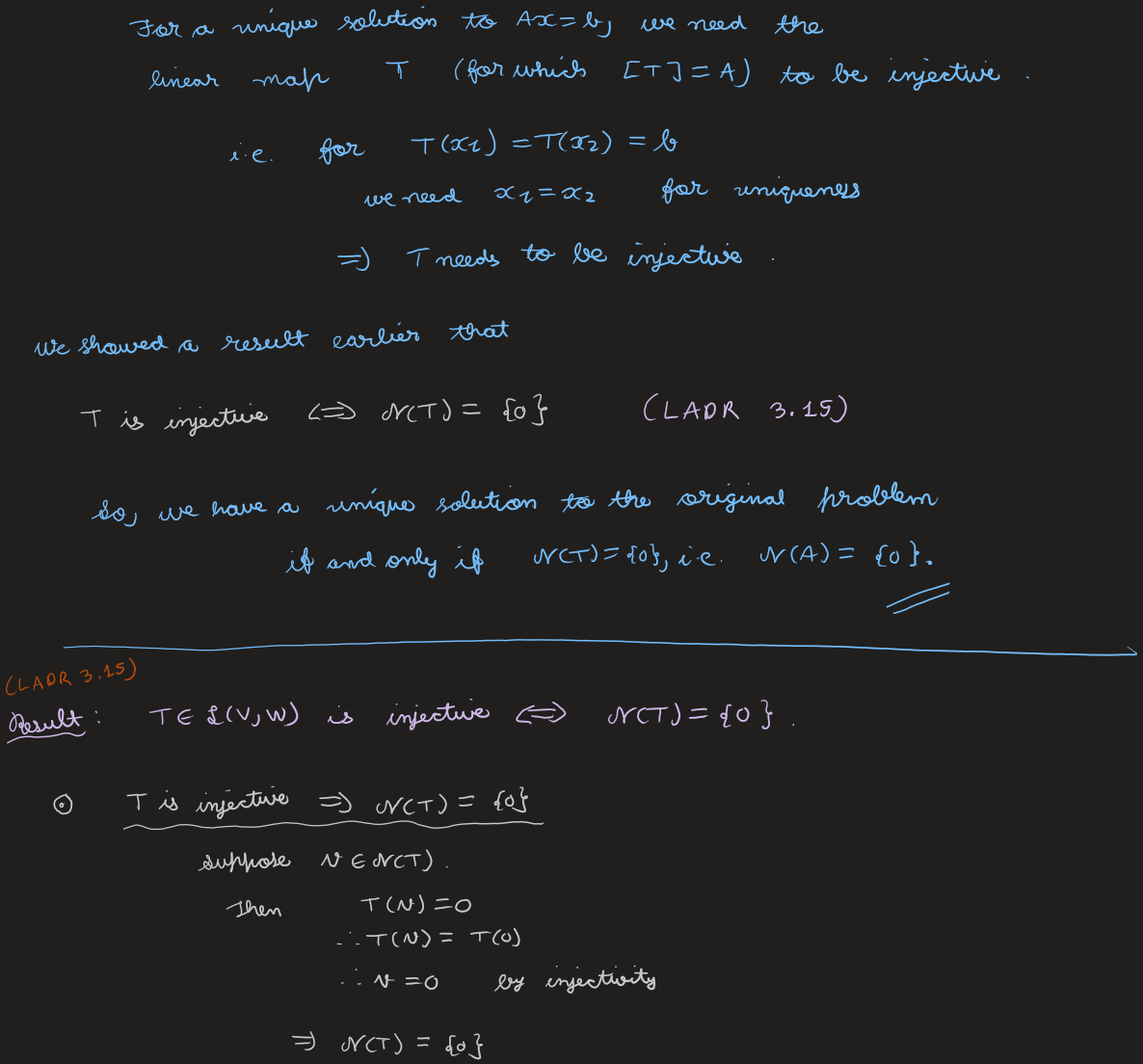
Uniqueness \( \iff \Null(A) = \{0\} \). A unique solution requires the map \( T \) (\( [T] = A \)) to be injective: \( T(x_1) = T(x_2) \Rightarrow x_1 = x_2 \). We showed earlier that \( T \) is injective \( \iff \Null(T) = \{0\} \) (LADR 3.15). So the normal equations have a unique solution iff \( \Null(A) = \{0\} \).
Result — LADR 3.15
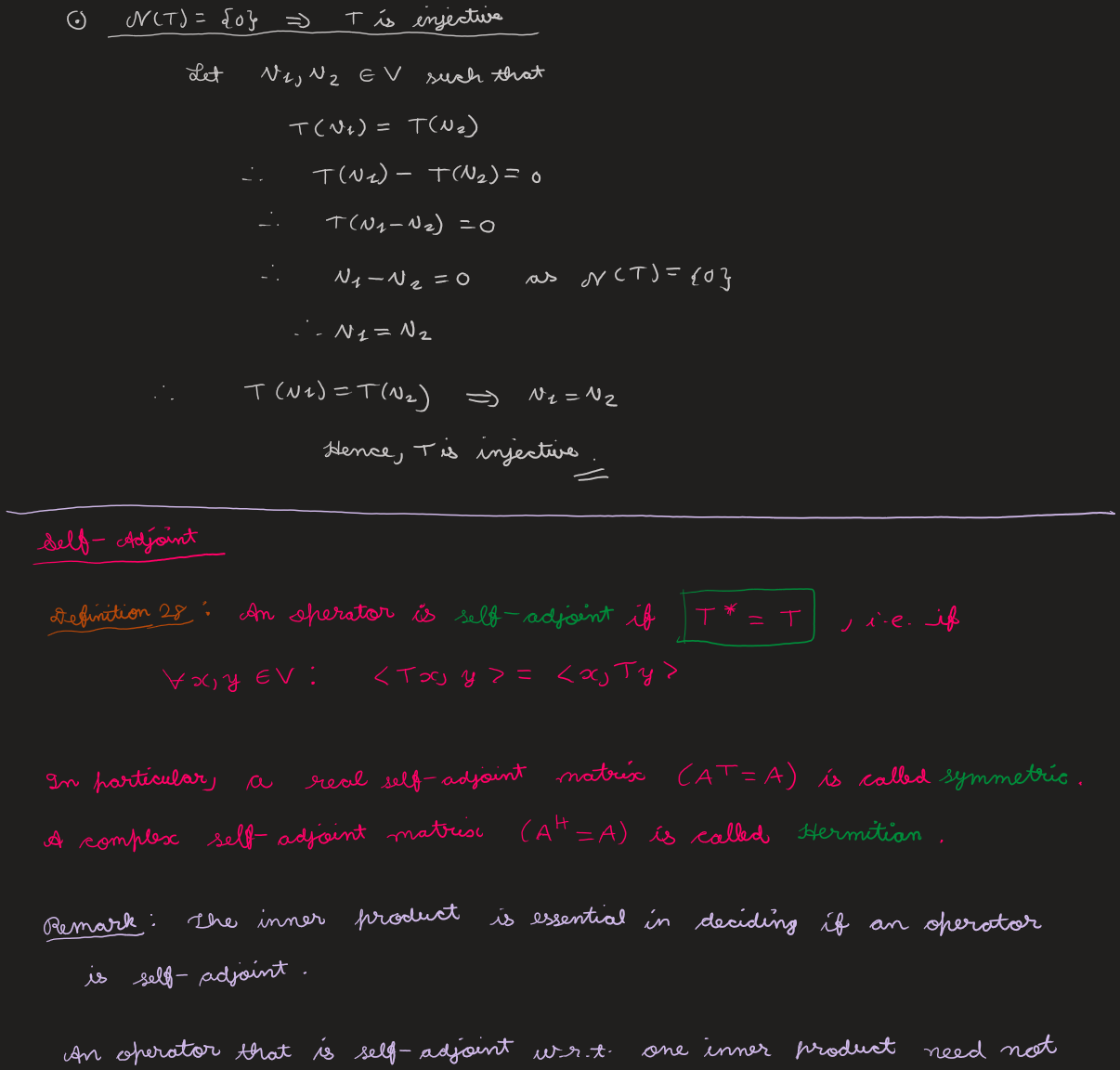
\( T \in \Lin(V, W) \) is injective \( \iff \Null(T) = \{0\} \). (\( \Rightarrow \)) If \( v \in \Null(T) \), then \( Tv = 0 = T(0) \Rightarrow v = 0 \). (\( \Leftarrow \)) If \( Tv_1 = Tv_2 \), then \( T(v_1 - v_2) = 0 \Rightarrow v_1 - v_2 = 0 \Rightarrow v_1 = v_2 \).
View original handwritten scans — Theorem 9 & proof, Ex 60–61, LADR 3.15 (pages 29–38)
Self-Adjoint Operators
Definition 28 — Self-adjoint
An operator is self-adjoint if \( T^* = T \), i.e. if \( \forall\, x, y \in V : \langle Tx, y\rangle = \langle x, Ty\rangle \). In particular, a real self-adjoint matrix (\( A\T = A \)) is called symmetric, and a complex self-adjoint matrix (\( A\herm = A \)) is called Hermitian.
Remark
The inner product is essential in deciding if an operator is self-adjoint. An operator that is self-adjoint w.r.t. one inner product need not be self-adjoint w.r.t. a different inner product.
Ex 62
Let \( P \in \Lin(V) \) be such that \( P^2 = P \). Prove that \( P \) is an orthogonal projector if and only if \( P \) is self-adjoint.
Solution
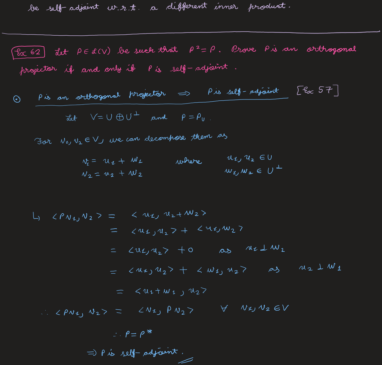
(\( \Rightarrow \)) Orthogonal projector \( \Rightarrow \) self-adjoint. This is Ex 57: with \( V = U \oplus U^{\perp} \), \( P = P_U \), and \( v_1 = u_1 + w_1 \), \( v_2 = u_2 + w_2 \), \[ \langle Pv_1, v_2\rangle = \langle u_1, u_2\rangle = \langle v_1, Pv_2\rangle, \] so \( P = P^* \).
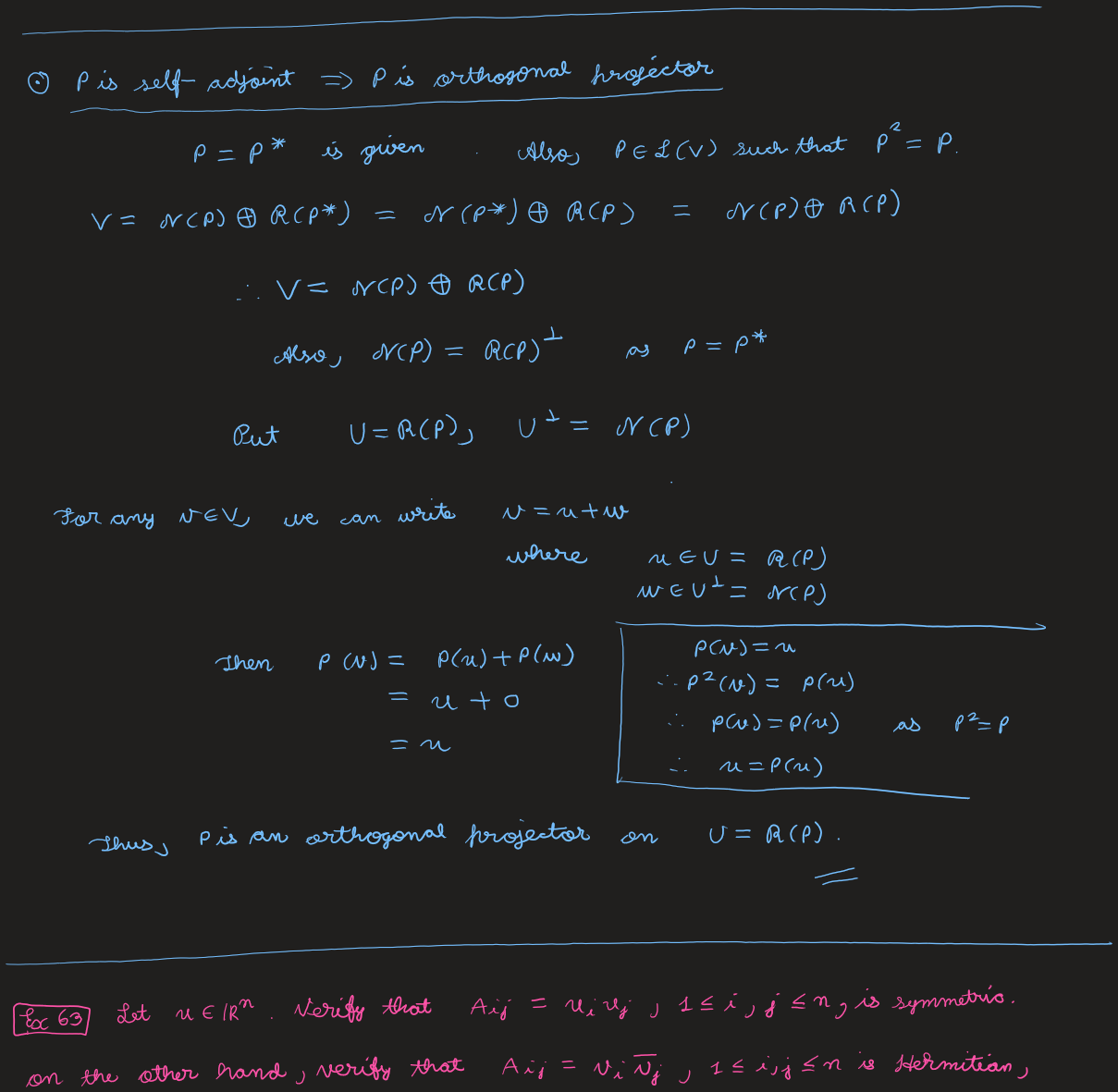
(\( \Leftarrow \)) Self-adjoint \( \Rightarrow \) orthogonal projector. Given \( P = P^* \) and \( P^2 = P \). Then \[ V = \Null(P) \oplus \Range(P^*) = \Null(P) \oplus \Range(P), \qquad \Null(P) = \Range(P)^{\perp}, \] using \( P = P^* \). Put \( U = \Range(P) \), \( U^{\perp} = \Null(P) \). For \( v = u + w \) (\( u \in U \), \( w \in U^{\perp} \)): any \( u \in \Range(P) \) satisfies \( P(u) = u \) (since \( u = P(x) \Rightarrow P(u) = P^2(x) = P(x) = u \)), and \( P(w) = 0 \). Hence \( P(v) = u \), so \( P \) is the orthogonal projector onto \( U = \Range(P) \).
Ex 63
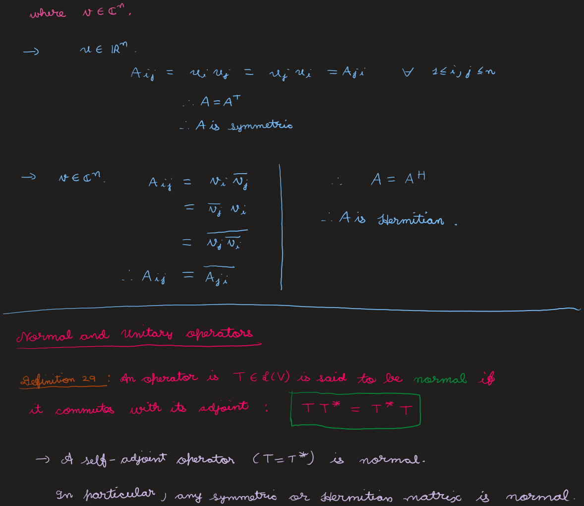
Let \( u \in \R^n \). Verify that \( A_{ij} = u_i u_j \) (\( 1 \le i, j \le n \)) is symmetric. For \( v \in \C^n \), verify that \( A_{ij} = v_i \bar v_j \) (\( 1 \le i, j \le n \)) is Hermitian.
Solution
Symmetric. \( A_{ij} = u_i u_j = u_j u_i = A_{ji} \ \forall\, i, j \), so \( A = A\T \).
Hermitian. \( A_{ij} = v_i \bar v_j = \bar v_j v_i = \overline{v_j \bar v_i} = \overline{A_{ji}} \ \forall\, i, j \), so \( A = A\herm \).
View original handwritten scans — self-adjoint operators, Def 28, Ex 62–63 (pages 38–41)
Normal & Unitary Operators
Definition 29 — Normal
An operator \( T \in \Lin(V) \) is said to be normal if it commutes with its adjoint: \[ TT^* = T^*T. \] A self-adjoint operator (\( T = T^* \)) is normal. In particular, any symmetric or Hermitian matrix is normal.
Definition 30 — Unitary
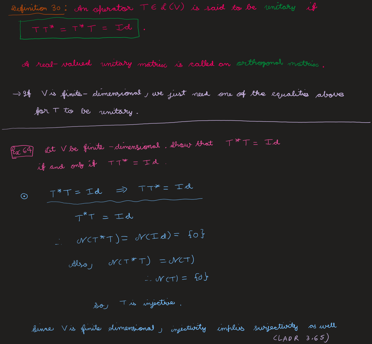
An operator \( T \in \Lin(V) \) is said to be unitary if \[ TT^* = T^*T = \mathrm{Id}. \] A real-valued unitary matrix is called an orthogonal matrix. If \( V \) is finite-dimensional, we just need one of the equalities above for \( T \) to be unitary.
Ex 64
Let \( V \) be finite-dimensional. Show that \( T^*T = \mathrm{Id} \) if and only if \( TT^* = \mathrm{Id} \).
Solution
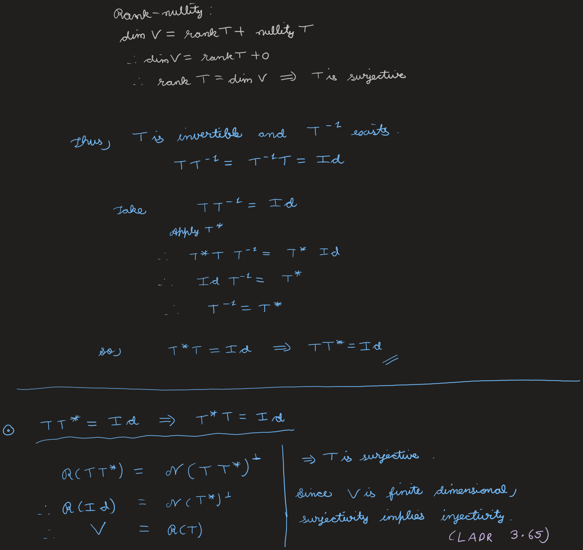
(\( \Rightarrow \)) \( T^*T = \mathrm{Id} \Rightarrow \Null(T^*T) = \{0\} \); but \( \Null(T^*T) = \Null(T) \), so \( \Null(T) = \{0\} \) and \( T \) is injective. In finite dimensions injectivity implies surjectivity (LADR 3.65), so by rank–nullity \( \rank T = \dim V \) and \( T \) is invertible. From \( TT^{-1} = \mathrm{Id} \), applying \( T^* \): \( T^*T\,T^{-1} = T^* \Rightarrow T^{-1} = T^* \), hence \( TT^* = \mathrm{Id} \).
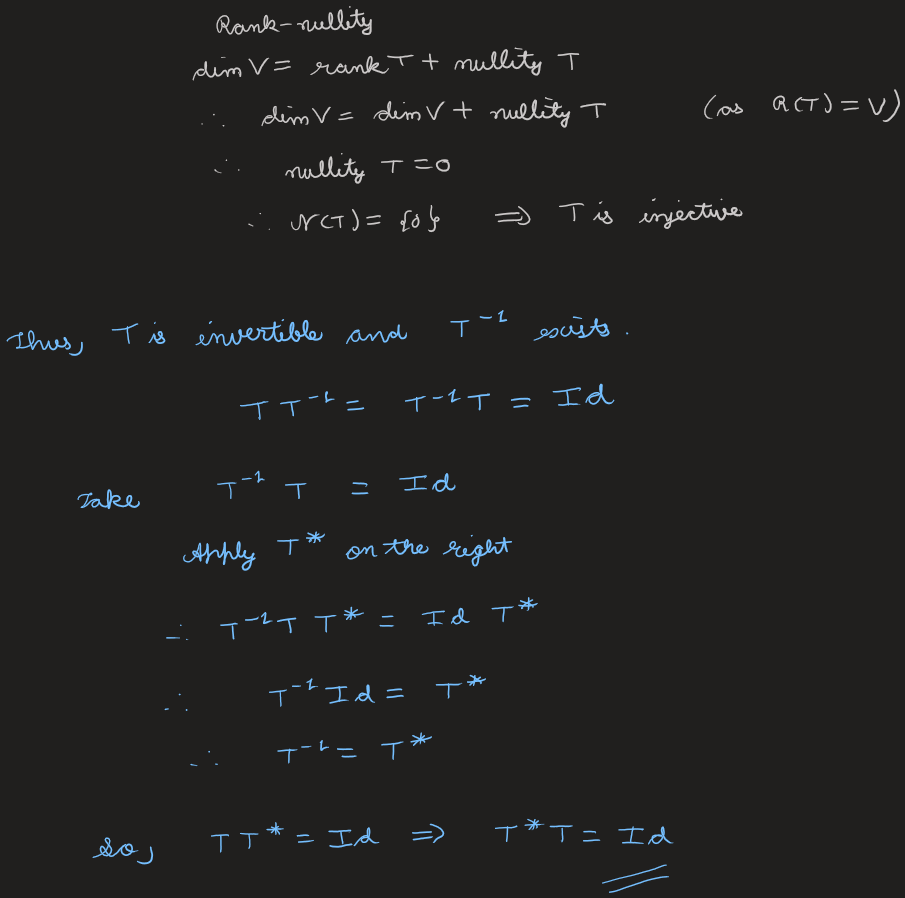
(\( \Leftarrow \)) \( TT^* = \mathrm{Id} \Rightarrow \Range(TT^*) = V \), and \( \Range(TT^*) = \Null(TT^*)^{\perp} = \Null(T^*)^{\perp} = \Range(T) \), so \( \Range(T) = V \) and \( T \) is surjective, hence (finite dimensions) bijective and invertible. From \( T^{-1}T = \mathrm{Id} \), applying \( T^* \) on the right: \( T^{-1}TT^* = T^* \Rightarrow T^{-1} = T^* \), hence \( T^*T = \mathrm{Id} \).
View original handwritten scans — normal & unitary operators, Def 29–30, Ex 64 (pages 41–44)
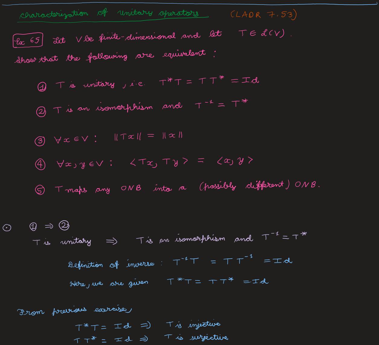
Characterization of Unitary Operators
Ex 65 — LADR 7.53
Let \( V \) be finite-dimensional and \( T \in \Lin(V) \). Show that the following are equivalent:
- \( T \) is unitary, i.e. \( T^*T = TT^* = \mathrm{Id} \);
- \( T \) is an isomorphism and \( T^{-1} = T^* \);
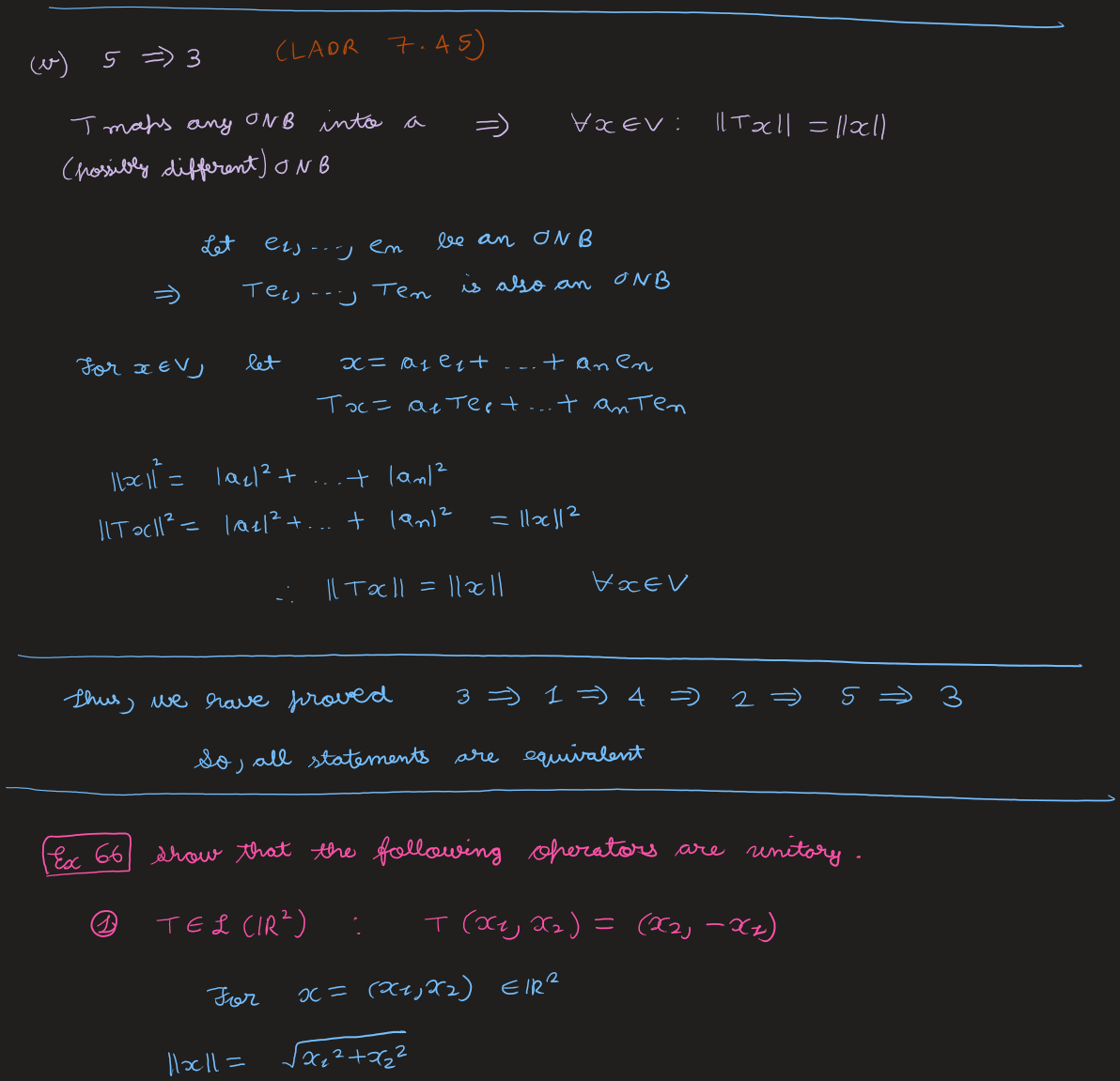
- \( \forall\, x \in V : \|Tx\| = \|x\| \) (isometry);
- \( \forall\, x, y \in V : \langle Tx, Ty\rangle = \langle x, y\rangle \);
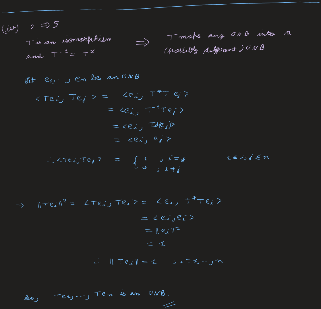
- \( T \) maps any ONB into a (possibly different) ONB.
Solution — cycle (1) ⟹ (2) ⟹ (3) ⟹ (4) ⟹ (5) ⟹ (1)
(1) \( \Rightarrow \) (2). \( T^*T = \mathrm{Id} \Rightarrow T \) injective and \( TT^* = \mathrm{Id} \Rightarrow T \) surjective (Ex 64); in finite dimensions \( T \) is an isomorphism. Applying \( T^{-1} \) to \( T^*T = \mathrm{Id} \) gives \( T^* = T^{-1} \).
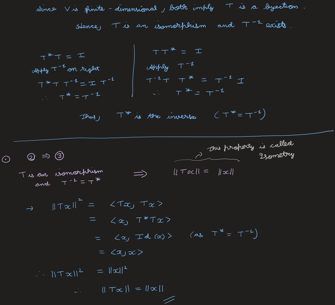
(2) \( \Rightarrow \) (3). \( \|Tx\|^2 = \langle Tx, Tx\rangle = \langle x, T^*Tx\rangle = \langle x, \mathrm{Id}(x)\rangle = \langle x, x\rangle \) (using \( T^* = T^{-1} \)), so \( \|Tx\| = \|x\| \).
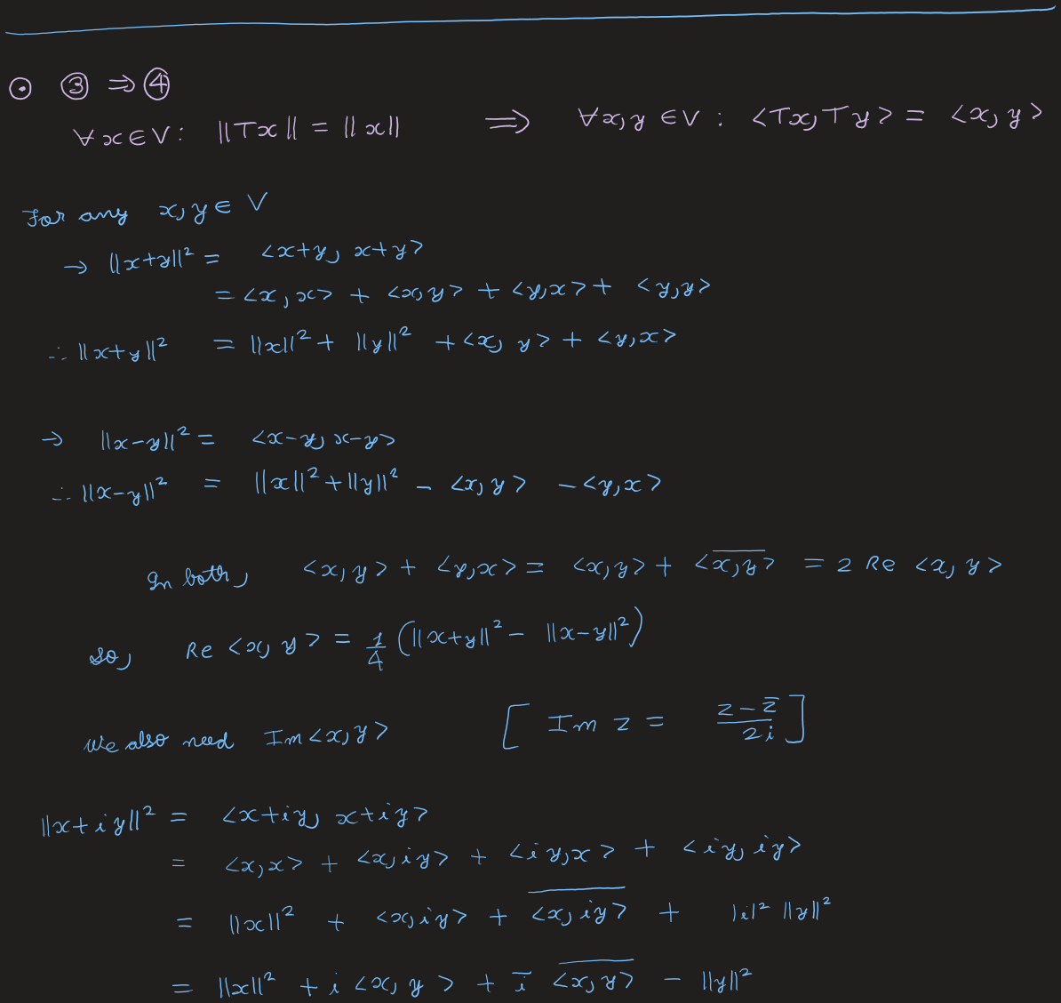
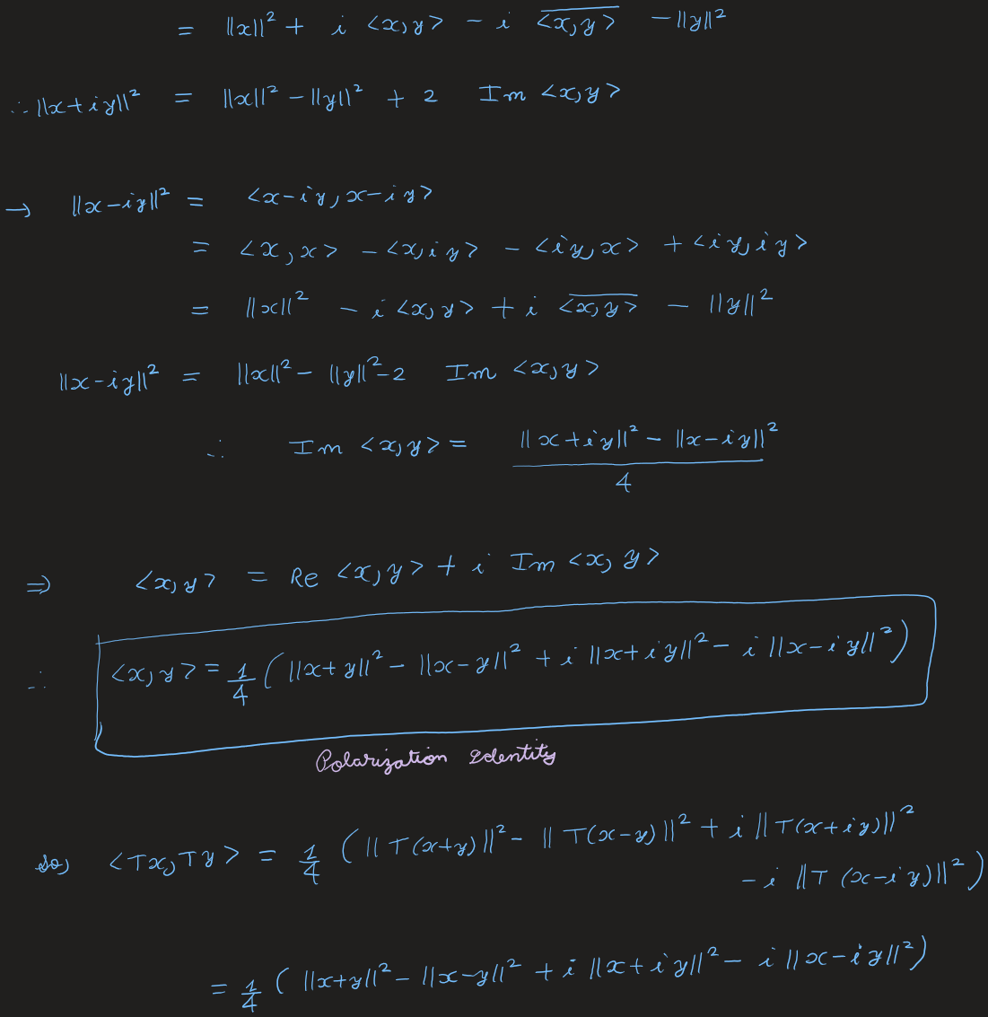
(3) \( \Rightarrow \) (4). By the polarization identity (below), the inner product is determined by the norm; since \( T \) preserves norms, \[\begin{aligned} \langle Tx, Ty\rangle &= \tfrac14\big(\|T(x+y)\|^2 - \|T(x-y)\|^2 - i\|T(x+iy)\|^2 + i\|T(x-iy)\|^2\big) \\ &= \tfrac14\big(\|x+y\|^2 - \|x-y\|^2 - i\|x+iy\|^2 + i\|x-iy\|^2\big) \\ &= \langle x, y\rangle. \end{aligned}\]
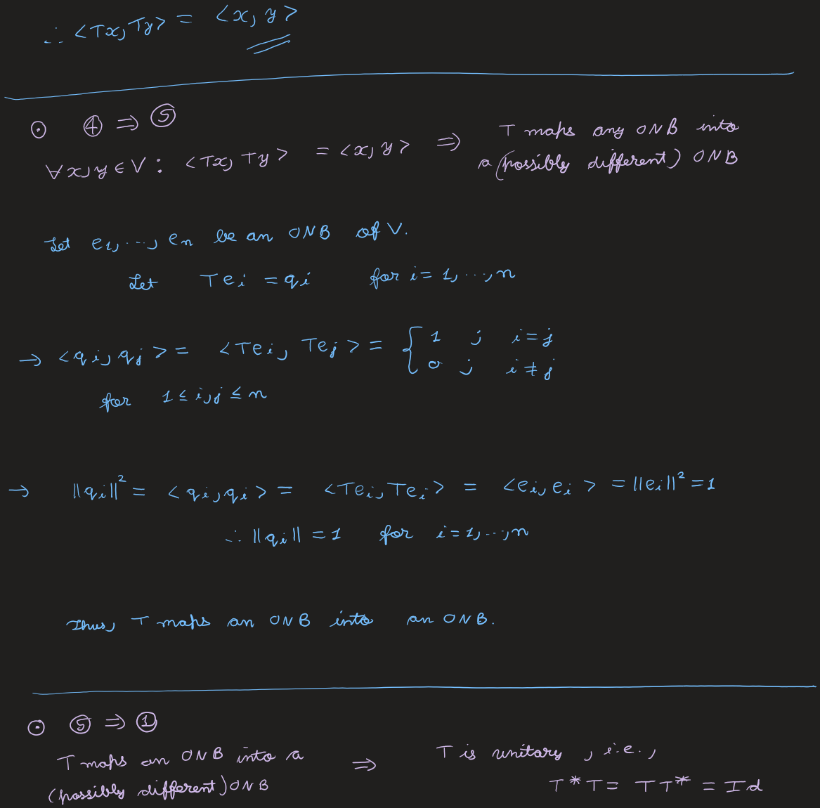
(4) \( \Rightarrow \) (5). Let \( e_1, \dots, e_n \) be an ONB and \( q_i = Te_i \). Then \( \langle q_i, q_j\rangle = \langle Te_i, Te_j\rangle = \langle e_i, e_j\rangle = \delta_{ij} \), and \( \|q_i\|^2 = \langle e_i, e_i\rangle = 1 \). So \( Te_1, \dots, Te_n \) is an ONB.
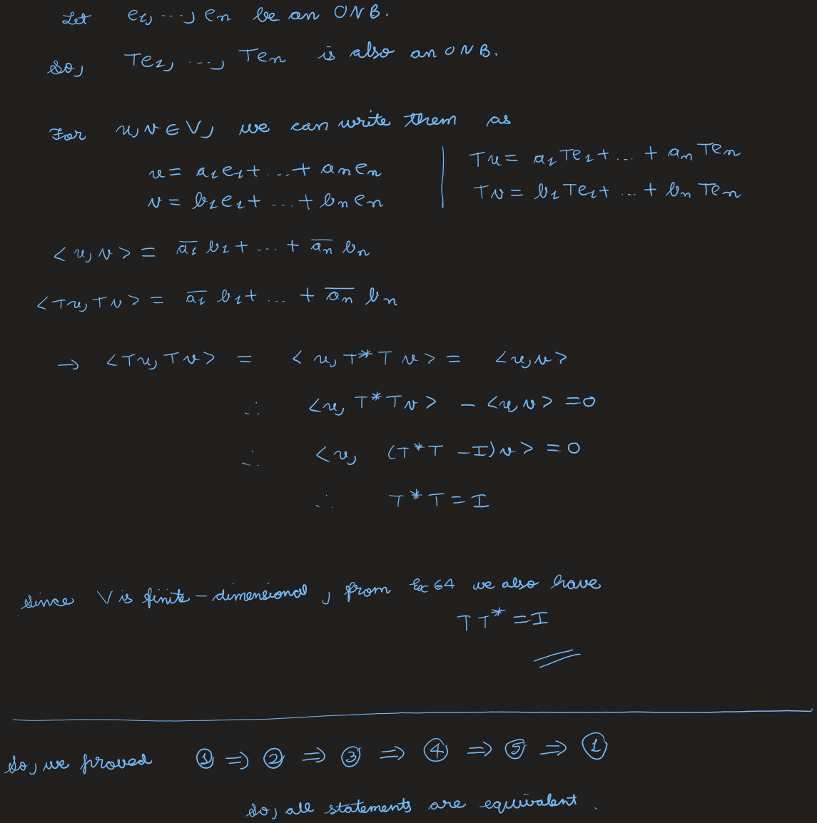
(5) \( \Rightarrow \) (1). Let \( e_1, \dots, e_n \) be an ONB, so \( Te_1, \dots, Te_n \) is too. For \( u = \sum a_i e_i \), \( v = \sum b_i e_i \), both \( \langle u, v\rangle \) and \( \langle Tu, Tv\rangle \) equal \( \bar a_1 b_1 + \dots + \bar a_n b_n \). Hence \( \langle u, (T^*T - I)v\rangle = 0 \ \forall\, u, v \Rightarrow T^*T = I \), and (Ex 64) \( TT^* = I \), so \( T \) is unitary.
Polarization Identity
From \( \|x \pm y\|^2 = \|x\|^2 + \|y\|^2 \pm (\langle x, y\rangle + \langle y, x\rangle) \) one gets \( \operatorname{Re}\langle x, y\rangle = \tfrac14(\|x+y\|^2 - \|x-y\|^2) \), and from the analogous \( \|x \pm iy\|^2 \) expansions \( \operatorname{Im}\langle x, y\rangle = \tfrac14(\|x-iy\|^2 - \|x+iy\|^2) \). Hence \[ \langle x, y\rangle = \tfrac14\big(\|x+y\|^2 - \|x-y\|^2 - i\|x+iy\|^2 + i\|x-iy\|^2\big). \]
Correction
The handwritten derivation writes \( \langle iy, iy\rangle = -\|y\|^2 \) (it is \( +\|y\|^2 \)) and flips the sign of \( \operatorname{Im}\langle x,y\rangle \), landing on the standard textbook identity \( \tfrac14(\dots + i\|x+iy\|^2 - i\|x-iy\|^2) \). That form assumes the inner product is conjugate-linear in the second slot. This course's convention is conjugate-linear in the first slot (Ch 4, Theorem 4: \( \langle u,w\rangle = \bar\alpha_1\beta_1 + \dots \)), under which the standard form computes \( \langle y, x\rangle \) instead. The imaginary signs are flipped above to match: e.g. with \( x = 1,\ y = i \), \( \langle x,y\rangle = \bar 1\cdot i = i \), which the corrected formula gives (the original yields \( -i \)). The same corrected signs are now used in the (3) ⟹ (4) step of Ex 65 above, which pass 1 had inadvertently left in the textbook (second-slot) form.
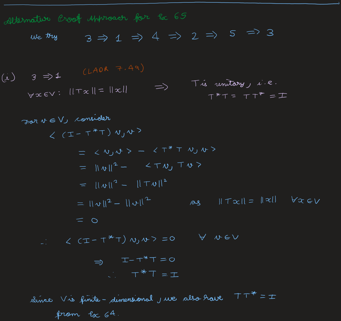
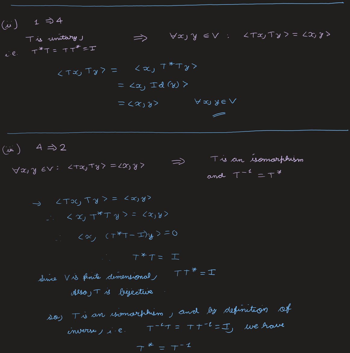
Alternative proof approach — cycle (3) ⟹ (1) ⟹ (4) ⟹ (2) ⟹ (5) ⟹ (3); LADR 7.45, 7.49
The genuinely different step is (3) \( \Rightarrow \) (1): for \( v \in V \), \[ \langle (I - T^*T)v, v\rangle = \langle v, v\rangle - \langle T^*Tv, v\rangle = \|v\|^2 - \|Tv\|^2 = 0 \quad \forall\, v \implies I - T^*T = 0, \] so \( T^*T = I \), and (Ex 64) \( TT^* = I \). The remaining implications mirror the cycle above.
View original handwritten scans — unitary characterization Ex 65, both proof routes & polarization identity (pages 45–54)
Examples of Unitary Operators
Ex 66
Show that the following operators are unitary.
- \( T \in \Lin(\R^2) \), \( T(x_1, x_2) = (x_2, -x_1) \).
- \( A \in \R^{2\times 2} \), \( A = \begin{bmatrix} \cos\theta & \sin\theta \\ -\sin\theta & \cos\theta \end{bmatrix} \).
- \( A \in \C^{2\times 2} \), \( A = \dfrac{1}{\sqrt 2}\begin{bmatrix} e^{i\theta} & -e^{-i\theta} \\ e^{i\theta} & e^{-i\theta} \end{bmatrix} \).
Solution
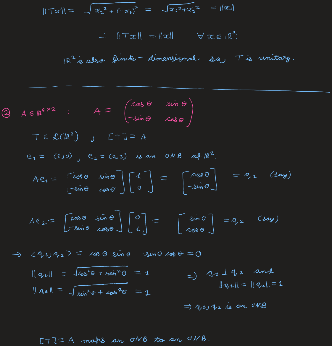
(1) For \( x = (x_1, x_2) \in \R^2 \), \( \|Tx\| = \sqrt{x_2^2 + (-x_1)^2} = \sqrt{x_1^2 + x_2^2} = \|x\| \). As \( \R^2 \) is finite-dimensional, \( T \) is unitary (isometry \( \Rightarrow \) unitary, Ex 65).
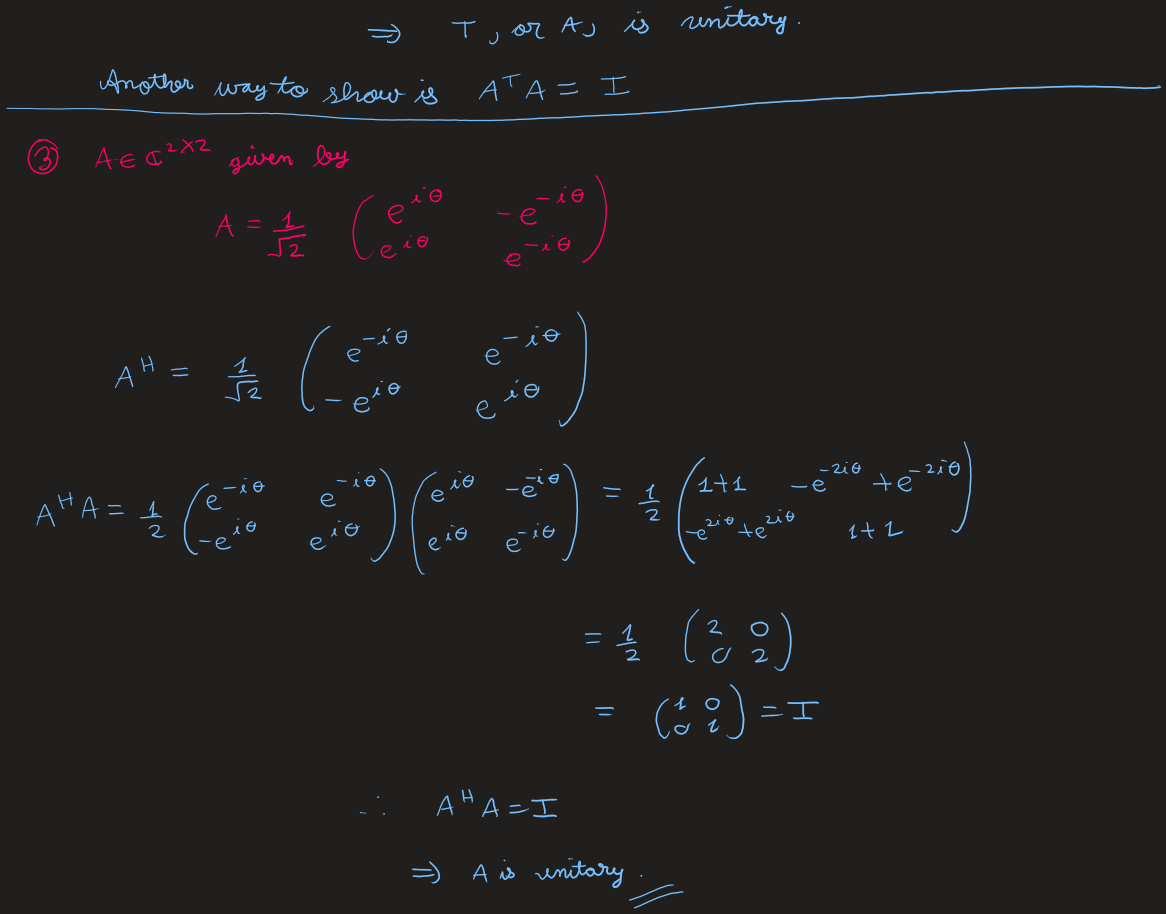
(2) With ONB \( e_1 = (1,0) \), \( e_2 = (0,1) \): \( Ae_1 = (\cos\theta, -\sin\theta) = q_1 \), \( Ae_2 = (\sin\theta, \cos\theta) = q_2 \). Then \( \langle q_1, q_2\rangle = \cos\theta\sin\theta - \sin\theta\cos\theta = 0 \) and \( \|q_1\| = \|q_2\| = \sqrt{\cos^2\theta + \sin^2\theta} = 1 \), so \( q_1, q_2 \) is an ONB. Thus \( A \) maps an ONB to an ONB, so \( A \) is unitary. (Equivalently, \( A\T A = I \).)
(3) Here \( A\herm = \dfrac{1}{\sqrt 2}\begin{bmatrix} e^{-i\theta} & e^{-i\theta} \\ -e^{i\theta} & e^{i\theta} \end{bmatrix} \), and \[ A\herm A = \frac12 \begin{bmatrix} e^{-i\theta} & e^{-i\theta} \\ -e^{i\theta} & e^{i\theta} \end{bmatrix}\begin{bmatrix} e^{i\theta} & -e^{-i\theta} \\ e^{i\theta} & e^{-i\theta} \end{bmatrix} = \frac12 \begin{bmatrix} 1+1 & -e^{-2i\theta} + e^{-2i\theta} \\ -e^{2i\theta} + e^{2i\theta} & 1+1 \end{bmatrix} = \frac12\begin{bmatrix} 2 & 0 \\ 0 & 2 \end{bmatrix} = I. \] So \( A\herm A = I \), hence \( A \) is unitary.
View original handwritten scans — unitary examples, Ex 66 (pages 54–56)